Making upset plots from GHRU data

Anthony Underwood

Introduction

UpSet diagrams visualizes complex intersections where the columns represent different combinations of factors across different sets of groups (rows). They are very helpful when looking at the different combinations of AMR determinants that may be responsible for resistance.

Getting and formatting the data

---

First get the relevant data sets

library(ghruR)
library(kableExtra)
epi_data <- ghruR::get_data_for_country(
  country_value = "India",
  type_value = "Epidemiological Metadata",
  user_email = "anthony.underwood@cgps.group")

## [1] "anthony.underwood@cgps.group"
## [1] "anthony.underwood@cgps.group"
## [1] "anthony.underwood@cgps.group"

epi_data <- ghruR::clean_data(epi_data)

ast_data <- ghruR::get_data_for_country(
  country_value = "India",
  type_value = "Antimicrobial Susceptibility Testing",
  user_email = "anthony.underwood@cgps.group")

## [1] "anthony.underwood@cgps.group"

acquired_amr_data <- ghruR::get_data_for_country(
  country_value = "India",
  type_value = "AMR Klebsiella pneumoniae",
  AMR_type = "acquired",
  user_email = "anthony.underwood@cgps.group")

## [1] "anthony.underwood@cgps.group"

point_amr_data <- ghruR::get_data_for_country(
  country_value = "India",
  type_value = "AMR Klebsiella pneumoniae",
  AMR_type = "point",
  user_email = "anthony.underwood@cgps.group")

## [1] "anthony.underwood@cgps.group"

mlst_data <- ghruR::get_data_for_country(
  country_value = "India",
  type_value = "MLST",
  user_email = "anthony.underwood@cgps.group")

## [1] "anthony.underwood@cgps.group"

Parsing the acquired AMR data

---

Convert the acquired AMR data to long format, annotate it and get the different data sets

# convert to long format
annotated_amr_data <- ghruR::annotate_amr_data(acquired_amr_data)
# filter data for those that have acquired the gene and have good pct_id match and ctg_cov
acquired_genes_present <- ghruR::filter_long_data(annotated_amr_data)
# filter by subclass
carbapenamases <- acquired_genes_present %>%
  dplyr::filter(subclass == "CARBAPENEM") %>%
  dplyr::select(`Sample id`, gene) %>%
  dplyr::rename(determinant = gene)

head(carbapenamases) %>% kable() %>% kable_styling() %>% scroll_box(width = "100%")

Sample id	determinant
G18250048	blaNDM-1
G18250048	blaOXA-181
G18250048	blaOXA-181
G18250088	blaNDM-1
G18250088	blaOXA-232
G18250088	blaOXA-232

esbls <- acquired_genes_present %>%
  dplyr::filter(subclass == "CEPHALOSPORIN") %>%
  dplyr::select(`Sample id`, gene) %>%
  dplyr::rename(determinant = gene) %>%
  dplyr::filter(
    str_starts(determinant, "blaCTX-M") |
    str_starts(determinant, "blaSHV") |
    str_starts(determinant, "blaTEM") |
     str_starts(determinant, "blaOXA")
  )
head(esbls) %>% kable() %>% kable_styling() %>% scroll_box(width = "100%")

Sample id	determinant
G18250048	blaCTX-M-15
G18250088	blaCTX-M-15
G18250088	blaOXA-1
G18250103	blaCTX-M-15
G18250103	blaOXA-1
G18250114	blaCTX-M-15

Parsing the point AMR data

---

Now handling point data, first get the mutations in assembled genes

annotated_point_amr_data <- ghruR::get_annotated_point_amr_data(point_amr_data, 'klebsiella', annotation_type = 'mutations')
# get mutations specific for carbapenems
carbapenam_specific_mutations <- annotated_point_amr_data %>%
  dplyr::filter(resistance == "carbapenem") %>% 
  select(-resistance)
head(carbapenam_specific_mutations) %>% kable() %>% kable_styling() %>% scroll_box(width = "100%")

Sample id	determinant
G18250048	ompK36_A217S
G18250048	ompK37_E244D
G18250048	ompK37_I128M
G18250048	ompK37_I70M
G18250048	ompK37_N230G
G18250088	ompK36_A217S

Now get the genes which were incomplete (partial or fragmented) and therefore possibly non-functional

annotated_point_amr_data <- ghruR::get_annotated_point_amr_data(point_amr_data, 'klebsiella', annotation_type = 'incomplete')
# get mutations specific for carbapenems
carbapenam_specific_incomplete_genes <- annotated_point_amr_data %>%
  dplyr::filter(resistance == "carbapenem") %>% 
  select(-resistance)
head(carbapenam_specific_incomplete_genes) %>% kable() %>% kable_styling() %>% scroll_box(width = "100%")

Sample id	determinant
G18251889	ompK36-absent
G18252053	ompK36-absent
G18252054	ompK36-partial
G18253166	ompK36-partial
G18253170	ompK36-absent
G18253171	ompK36-partial

For simplicity in the plots convert both of these to be either gene-mutation or gene-incomplete

carbapenam_specific_mutations %<>% dplyr::mutate(determinant = stringr::str_replace(determinant, "_.+$", "-mutation")) %>%
  dplyr::distinct(`Sample id`, determinant)
head(carbapenam_specific_mutations) %>% kable() %>% kable_styling() %>% scroll_box(width = "100%")

Sample id	determinant
G18250048	ompK36-mutation
G18250048	ompK37-mutation
G18250088	ompK36-mutation
G18250088	ompK37-mutation
G18250103	ompK36-mutation
G18250103	ompK37-mutation

carbapenam_specific_incomplete_genes %<>% dplyr::mutate(determinant = stringr::str_replace(determinant, "-.+$", "-incomplete")) %>%
  dplyr::distinct(`Sample id`, determinant)
head(carbapenam_specific_incomplete_genes) %>% kable() %>% kable_styling() %>% scroll_box(width = "100%")

Sample id	determinant
G18251889	ompK36-incomplete
G18252053	ompK36-incomplete
G18252054	ompK36-incomplete
G18253166	ompK36-incomplete
G18253170	ompK36-incomplete
G18253171	ompK36-incomplete

Combining all the dataframes

---

Produce a final dataframe from the acquired and point dataframes with determinants putatively involved in carbapenem resistance

This involves binding the rows and combining multiple determinants for the same sample into one by joining them into a list (for the ggupset function) using the group_by and summarise functions from the the dplyr package

#combine all determinants
all_potential_CR_determinants <-
  rbind(carbapenamases, esbls, carbapenam_specific_mutations, carbapenam_specific_incomplete_genes)

# merge multiple instances
all_potential_CR_determinants  %<>% dplyr::group_by(`Sample id`) %>%
  dplyr::summarise(determinant = list(determinant))

head(all_potential_CR_determinants) %>% kable() %>% kable_styling() %>% scroll_box(width = "100%")

Sample id	determinant
G18250048	blaNDM-1 , blaOXA-181 , blaOXA-181 , blaCTX-M-15 , ompK36-mutation, ompK37-mutation
G18250088	blaNDM-1 , blaOXA-232 , blaOXA-232 , blaCTX-M-15 , blaOXA-1 , ompK36-mutation, ompK37-mutation
G18250103	blaNDM-1 , blaOXA-232 , blaOXA-232 , blaCTX-M-15 , blaOXA-1 , ompK36-mutation, ompK37-mutation
G18250104	ompK36-mutation, ompK37-mutation
G18250114	blaNDM-1 , blaCTX-M-15 , blaOXA-1 , ompK36-mutation, ompK37-mutation
G18250122	blaNDM-1 , blaCTX-M-15 , blaOXA-1 , ompK36-mutation, ompK37-mutation

Filtering out samples without relevant loci

• filter out those without a carbapenamase
• Filter out those that have no beta lactamase and those that have a potential ESBL without a porin mutation

all_potential_CR_determinants %<>%
  dplyr::filter(str_detect(determinant, "bla"))

# filter out those with only ESBL but no OmpK mutations
all_potential_CR_determinants %<>%
  dplyr::filter(!
                  (
                    (
                      str_detect(determinant, "blaCTX-M") |
                      str_detect(determinant, "blaSHV") |
                      str_detect(determinant, "blaTEM") |
                      str_detect(determinant, "blaOXA")
                    ) &
                      !str_detect(determinant, "ompK")
                  )
  )
head(all_potential_CR_determinants) %>% kable() %>% kable_styling() %>% scroll_box(width = "100%")

Sample id	determinant
G18250048	blaNDM-1 , blaOXA-181 , blaOXA-181 , blaCTX-M-15 , ompK36-mutation, ompK37-mutation
G18250088	blaNDM-1 , blaOXA-232 , blaOXA-232 , blaCTX-M-15 , blaOXA-1 , ompK36-mutation, ompK37-mutation
G18250103	blaNDM-1 , blaOXA-232 , blaOXA-232 , blaCTX-M-15 , blaOXA-1 , ompK36-mutation, ompK37-mutation
G18250114	blaNDM-1 , blaCTX-M-15 , blaOXA-1 , ompK36-mutation, ompK37-mutation
G18250122	blaNDM-1 , blaCTX-M-15 , blaOXA-1 , ompK36-mutation, ompK37-mutation
G18251889	blaOXA-232 , blaOXA-232 , blaCTX-M-15 , ompK37-mutation , ompK36-incomplete

Plotting the data

---

Use the ggupset library to plot the data

library(ggupset)
# Find unique determinants to become the set labels
unique_determinants <- rbind(carbapenamases, esbls, carbapenam_specific_mutations, carbapenam_specific_incomplete_genes) %>%
  dplyr::distinct(determinant) %>%
  dplyr::arrange(determinant) %>%
  dplyr::pull(determinant)

# make the upset plot
upset_plot <- all_potential_CR_determinants %>%
  ggplot(aes(x=determinant)) +
  geom_bar() +
  scale_x_upset(order_by = "freq", sets = unique_determinants)

upset_plot

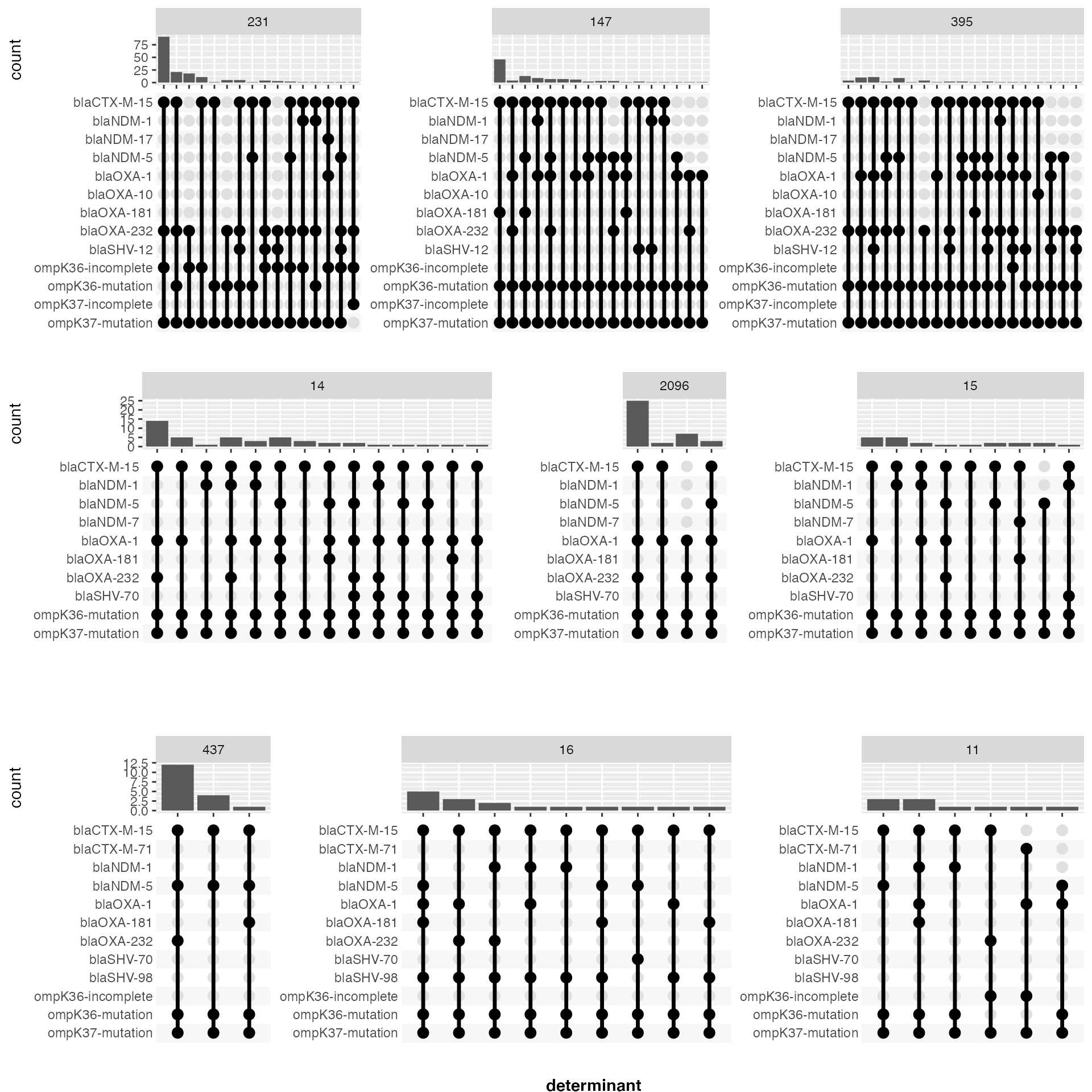
Breaking it down by ST

---

library(cowplot)
library(forcats)
all_potential_CR_determinants_and_ST <- all_potential_CR_determinants %>%
  dplyr::left_join(mlst_data %>% dplyr::select(`Sample id`, ST), by = "Sample id") 

num <- 9
most_frequent_STs <- all_potential_CR_determinants_and_ST %>%
  dplyr::select(ST) %>% dplyr::count(ST) %>%
  dplyr::arrange(desc(n)) %>% dplyr::slice_max(n, n = num) %>%
  dplyr::pull(ST)

plots = list()
plot_index <- 0
for (start in seq(1,9, by =3)){
  plot_index <- plot_index + 1

  end <- start + 2
  selected_STs <- most_frequent_STs[start:end]
  data_for_STs <- all_potential_CR_determinants_and_ST %>% dplyr::filter(ST %in% selected_STs)

  determinants_for_STs <- data_for_STs %>%
    unnest(cols = c(determinant)) %>%
    dplyr::distinct(determinant) %>%
    dplyr::arrange(determinant) %>%
    dplyr::pull(determinant)

  upset_plot_for_STs <-  data_for_STs %>%
    mutate(ST = fct_relevel(ST, selected_STs)) %>%
    ggplot(aes(x = determinant)) +
    geom_bar() +
    theme(plot.title = element_text(size = 20, face = "bold")) +
    facet_grid(cols = vars(ST), scales = "free_x", space = "free", drop = FALSE) +
    ggeasy::easy_labs(x = "") +
    scale_x_upset(order_by = "freq", sets = determinants_for_STs) +
    theme(panel.spacing.x=unit(6, "lines"))

  plots[[plot_index]] <- upset_plot_for_STs
}

plot_grid <- cowplot::plot_grid(plotlist = plots, align = "h", ncol = 1) +
  cowplot::draw_figure_label(label = "determinant", position = "bottom", font = "bold")

plot_grid