Making plots from GHRU data

Introduction

This vignette will demonstrate how to use some of the inbuilt GHRU R functions to plot data

Getting the required data

For these plots we will need epi data, MLST data and AMR data.

library(ghruR)
library(kableExtra)
epi_data <- ghruR::get_data_for_country(
  country_value = "India",
  type_value = "Epidemiological Metadata",
  user_email = "anthony.underwood@cgps.group")

## [1] "anthony.underwood@cgps.group"
## [1] "anthony.underwood@cgps.group"
## [1] "anthony.underwood@cgps.group"

epi_data <- ghruR::clean_data(epi_data)

mlst_data <- ghruR::get_data_for_country(
  country_value = "India",
  type_value = "MLST",
  user_email = "anthony.underwood@cgps.group")

## [1] "anthony.underwood@cgps.group"

amr_data <- ghruR::get_data_for_country(
  country_value = "India",
  type_value = "AMR Klebsiella pneumoniae",
  AMR_type = "acquired",
  user_email = "anthony.underwood@cgps.group")

## [1] "anthony.underwood@cgps.group"

Basic stats

# Select just the data for which we have AMR data
kpn_ids <- amr_data %>% pull(`Sample id`)
combined_data <- epi_data %>% 
  dplyr::filter(`Sample id` %in% kpn_ids) %>% 
  left_join(mlst_data, by = 'Sample id')
# Show some basic stats
samples_per_sentinel_site <- count_samples_by_sentinel_site(combined_data)
samples_per_sentinel_site %>% kable() %>% kable_styling() %>% scroll_box(width = "100%")

Sentinel Site Code	Sample Count
AIIMSJ	19
APH	5
BCH	258
BCR	9
CMC	8
IGIMS	21
IPH	1
JAY	70
JIP	55
KGMU	9
KMC	28
KMN	1
LPL	3
MEDQ	2
MIMS	5
NIM	5
PRIM	7
RBH	7
RRM	13
SDU	5
SMF	5
SMS	7
TSRM	6
UTK	29
VPC	64

Plotting ST data

Plot all STs ordered by count

st_counts <- ghruR::count_sts(combined_data)
st_plot <- plot_sts(st_counts, order_by_count = TRUE)
print(st_plot)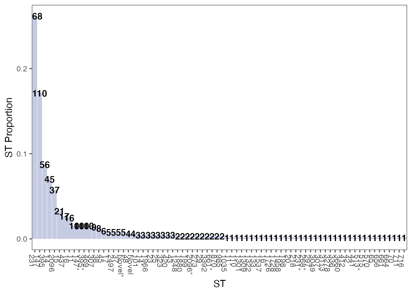

Plot top 10 most frequent STs ordered by count

most_frequent_sts <- count_most_frequent_sts(st_counts)
st_plot <- plot_sts(most_frequent_sts, order_by_count = TRUE)
print(st_plot)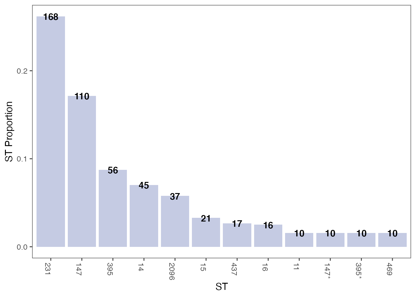

Plot most frequent STs by Sentinel Site

st_counts_by_sentinel_site <- count_sts_by_sentinel_site(combined_data)
most_frequent_st_counts_by_sentinel_site <- count_most_frequent_sts_per_sentinel_site(st_counts_by_sentinel_site, per_sentinel_site = 2)
plot_most_frequent_sentinel_site_sts(most_frequent_st_counts_by_sentinel_site)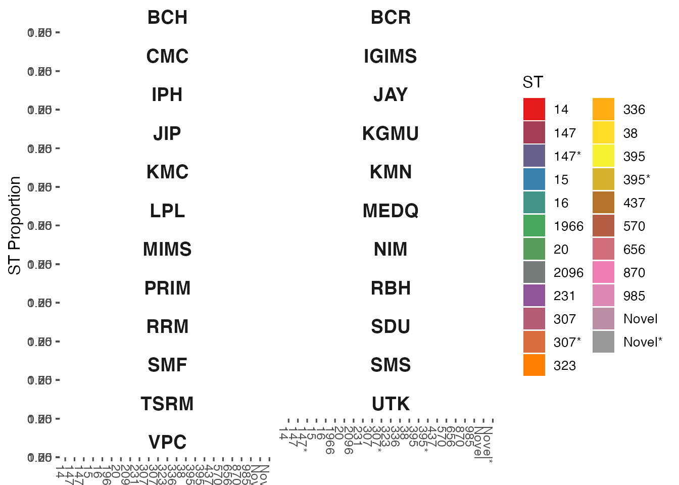

Plotting AMR data

First converting the amr data to long format and annotating with NCBI metadata and then plotting selected drug classes

# convert to long format
annotated_amr_data <- ghruR::annotate_amr_data(amr_data)
# filter data
annotated_amr_data <- ghruR::filter_long_data(annotated_amr_data)
# add Sentinel Site Code
annotated_amr_data  %<>% left_join(
  epi_data %>% select(`Sample id`, `Sentinel Site Code`),
  by = 'Sample id'
)
#  select drug classes
selected_drug_subclasses <- c("BETA-LACTAM", "CEPHALOSPORIN", "CARBAPENEM")

subclass_counts_by_sentinel_site <- ghruR::count_AMR_subclasses_by_sentinel_site(
  annotated_amr_data,
  samples_per_sentinel_site,
  selected_drug_subclasses
)
amr_subclasses_plot <- ghruR::plot_AMR_subclasses_by_sentinel_site(subclass_counts_by_sentinel_site)

Make a plot looking at the distribution of gene families. Combine them together

gene_family_counts_by_sentinel_site <- ghruR::count_gene_families_by_sentinel_site(
  annotated_amr_data,
  subclass_counts_by_sentinel_site,
  selected_drug_subclasses)

gene_family_dot_plot <- ghruR::dot_plot_gene_family_counts_by_sentinel_site(gene_family_counts_by_sentinel_site)
cowplot::plot_grid(amr_subclasses_plot, gene_family_dot_plot,ncol =1, align="v", rel_heights = c(1, 3))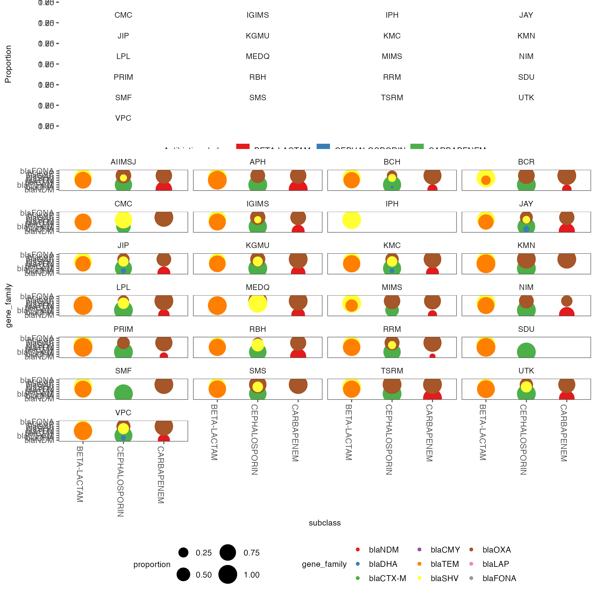

It is important to look at the gene alleles responsible for resistance. Here looking at just cephalosporin and carbapenem

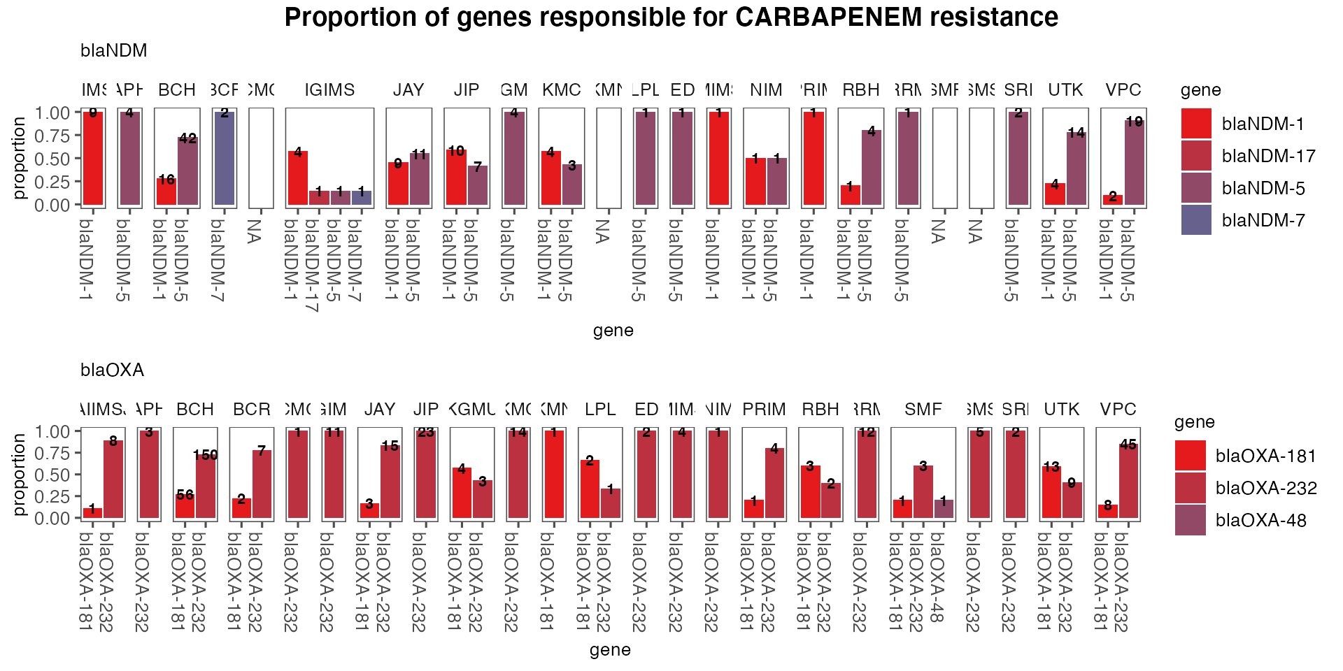
drug_subclasses <- c('CEPHALOSPORIN', 'CARBAPENEM')
allele_counts_by_sentinel_site <- ghruR::count_alleles_by_sentinel_site(
  annotated_amr_data,
  gene_family_counts_by_sentinel_site,
  drug_subclasses
)
allele_counts_plots <- ghruR::plot_allele_counts_by_sentinel_site(
  allele_counts_by_sentinel_site,
  drug_subclasses
)

print(allele_counts_plots[[1]])

print(allele_counts_plots[[2]])

Anthony Underwood