unPC Analysis
Che-Wei Chang
2021-10-15
Last updated: 2022-01-18
Checks: 7 0
Knit directory: Barley1kGBS_Proj/
This reproducible R Markdown analysis was created with workflowr (version 1.6.2). The Checks tab describes the reproducibility checks that were applied when the results were created. The Past versions tab lists the development history.
Great! Since the R Markdown file has been committed to the Git repository, you know the exact version of the code that produced these results.
Great job! The global environment was empty. Objects defined in the global environment can affect the analysis in your R Markdown file in unknown ways. For reproduciblity it's best to always run the code in an empty environment.
The command set.seed(20210831) was run prior to running the code in the R Markdown file. Setting a seed ensures that any results that rely on randomness, e.g. subsampling or permutations, are reproducible.
Great job! Recording the operating system, R version, and package versions is critical for reproducibility.
Nice! There were no cached chunks for this analysis, so you can be confident that you successfully produced the results during this run.
Great job! Using relative paths to the files within your workflowr project makes it easier to run your code on other machines.
Great! You are using Git for version control. Tracking code development and connecting the code version to the results is critical for reproducibility.
The results in this page were generated with repository version da73ff9. See the Past versions tab to see a history of the changes made to the R Markdown and HTML files.
Note that you need to be careful to ensure that all relevant files for the analysis have been committed to Git prior to generating the results (you can use wflow_publish or wflow_git_commit). workflowr only checks the R Markdown file, but you know if there are other scripts or data files that it depends on. Below is the status of the Git repository when the results were generated:
Ignored files:
    Ignored:    .Rhistory
    Ignored:    .Rproj.user/
    Ignored:    analysis/GenomeEnvAssociation_cache/
    Ignored:    analysis/GenomicVarPartitioning_cache/
    Ignored:    analysis/PreprocessEnvData_cache/

Untracked files:
    Untracked:  VennDiagram2022-01-18_16-08-05.log
    Untracked:  VennDiagram2022-01-18_16-10-17.log
Note that any generated files, e.g. HTML, png, CSS, etc., are not included in this status report because it is ok for generated content to have uncommitted changes.
These are the previous versions of the repository in which changes were made to the R Markdown (analysis/unPC.rmd) and HTML (public/unPC.html) files. If you've configured a remote Git repository (see ?wflow_git_remote), click on the hyperlinks in the table below to view the files as they were in that past version.
| File | Version | Author | Date | Message |
|---|---|---|---|---|
| html | 5f53139 | Che-Wei Chang | 2022-01-18 | Build site. |
| Rmd | 597a627 | Che-Wei Chang | 2021-11-30 | update analyses. unPC, ResistanceGA and GO enrichment |
| html | 597a627 | Che-Wei Chang | 2021-11-30 | update analyses. unPC, ResistanceGA and GO enrichment |
About unPC
unPC was proposed by House and Hahn (2017; https://doi.org/10.1111/1755-0998.12747) that is used for visualizing unusual patterns of genetic differentiation across a landscape.
The unPC score of a pair of subpopulations is calculated as the PCA-based genetic distances divided by geographic distance. The PCA-based genetic distance are computed as Euclidean distance between the PCA coordinates for each pair of populations. The PCA coordinates of populations are obtained by averaging the PCA coordinates (the 1st and 2nd PC dimensions) of individuals in each population.
Preparation of required data
rm(list = ls())
source("./code/Rfunctions.R")
library(MASS)
library(rnaturalearth)
library(raster)
library(rgdal)
library(mapplots)
library(scales)
library(rcompanion)
library(vcfR)
library(unPC)
vcf <- read.vcfR("/home/cheweichang/barley/WildBarleyGBS/Formal_PopGen_Analysis/GenotypicData/2020-04-07-GBS_191B1K+53KS_1st+2nd_batches_58geogroup_indmis0.1_indhet0.05_19601SNP_maf0.01_snpmis0.1_rm_het_LDprune_LDprune0.1.vcf.gz")
Xmat <- vcf_to_nummatrix(vcf = vcf)
impX <- t(apply(Xmat,1,function(x){
  x[is.na(x)] <- mean(x, na.rm = T)
  return(x)
}))

barley.pc <- svd(t(impX))

# set color codes
mycol <- alpha(c('#e41a1c','#377eb8','#4daf4a', '#ffffbf'), alpha = 0.8)


ind.ID <- colnames(impX)
clusters <- as.numeric(gsub(sapply(strsplit(colnames(impX), split = "_"), function(x){x[1]}), pattern = "Group", replacement = ""))

# `svd_to_unPCfile` is a customized function to convert SVD output to the input format of unPC
svd_to_unPCfile(pc = barley.pc, ind.ID = colnames(impX), clusters = as.numeric(gsub(sapply(strsplit(colnames(impX), split = "_"), function(x){x[1]}), pattern = "Group", replacement = ""))
                , file.n = "./output/unPC_PC_input.evec",K = 10)


## load geographic coordinates
geo <- read.table("./data/geo_coordinates_244accessions.tsv", header = T, stringsAsFactors = F)

## calculate mean geographic coordinates of samples from each deme
grp.coord <- cbind(tapply(geo$Longitude, INDEX = geo$GeoGroup, mean), tapply(geo$Latitude, INDEX = geo$GeoGroup, mean))

coord.out <- grp.coord[match(geo$GeoGroup,rownames(grp.coord)),]
write.table(coord.out[,c(2,1)], file = "./output/unPC_coord_input.txt", row.names = F, col.names = F)

# calculate ancestry coefficients
alsQ <- alstructure::alstructure(Xmat)$Q_hat
grp.Q <- apply(t(alsQ), 2, function(x){tapply(x, INDEX = geo$GeoGroup, mean)})
Run unPC
setwd("./output")
unPC::unPC(inputToProcess = "./unPC_PC_input.evec", geogrCoords = "./unPC_coord_input.txt",
           plotWithMap = TRUE, roundEarth = TRUE, outputPrefix = "191B1K+53KS_unPC_visualization")

unpcout <- readRDS("191B1K+53KS_unPC_visualization_pairwiseDistCalc_unPC.rds")
Box Cox transformation
trans.unPC <- boxcox(unpcout$ratioPCToGeogrDist ~ 1, lambda = seq(-6,6,0.01))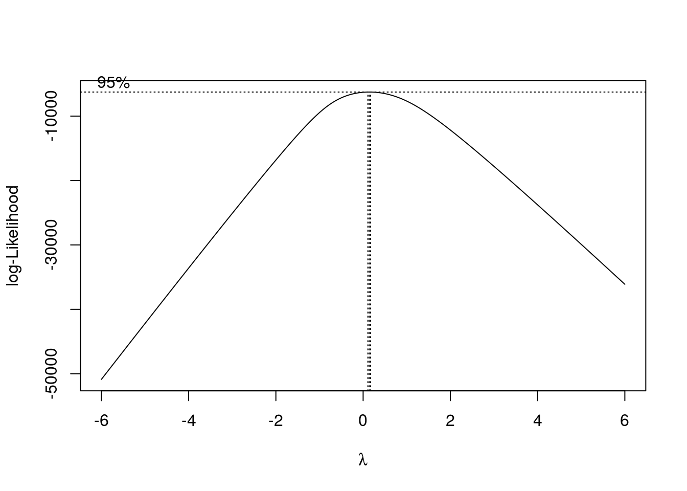
| Version | Author | Date |
|---|---|---|
| 597a627 | Che-Wei Chang | 2021-11-30 |
lambda <- trans.unPC$x[which.max(trans.unPC$y)]
unPC.boxcox <- (unpcout$ratioPCToGeogrDist^lambda - 1)/lambda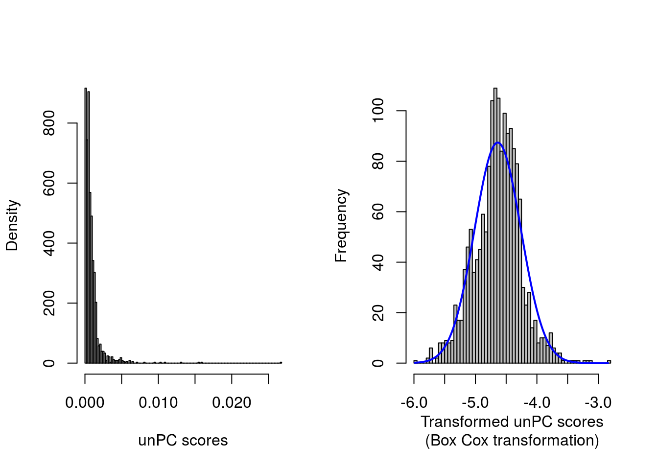
| Version | Author | Date |
|---|---|---|
| 597a627 | Che-Wei Chang | 2021-11-30 |
Population pairs with significantly unPC scores
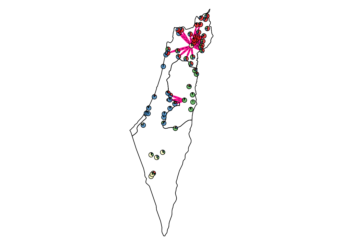
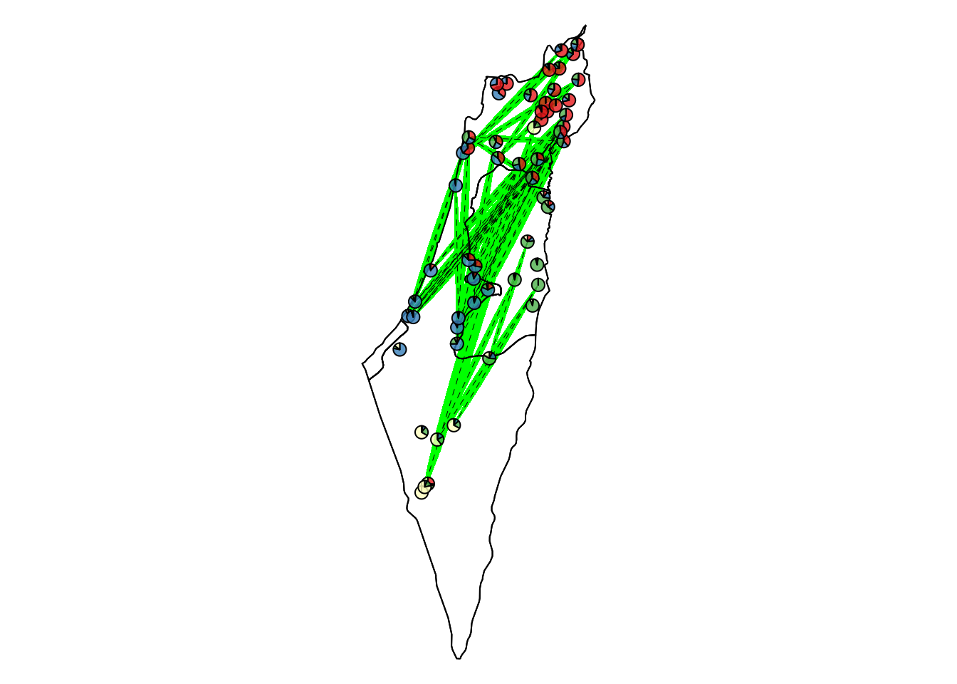
Outlier tests were carried out by a customized function plot.unPC. This function was modified from the unPC (House and Hahn. 2017). In this function, unPC scores are first normalized with scale and the corresponding probability cumulative densities are obtained with pt function. Then, unPC scores higher and lower than the significant threshold are regarded as population pairs violating the isolation-by-distance pattern. Here, we selected the 2.5% and 97.5% of Student's t distribution as significant thresholds.
Higher than the top 2.5% threshold
Comparisons with unPC scores higher than the top 2.5% threshold that indicates a significantly low genetic similarity over a short geographical distance.
| Version | Author | Date |
|---|---|---|
| 597a627 | Che-Wei Chang | 2021-11-30 |
Lower than the bottom 2.5% threshold
Comparisons with unPC scores lower than the bottom 2.5% threshold that indicates a significantly high genetic similarity over a long geographical distance.
| Version | Author | Date |
|---|---|---|
| 597a627 | Che-Wei Chang | 2021-11-30 |
sessionInfo()R version 3.6.0 (2019-04-26)
Platform: x86_64-pc-linux-gnu (64-bit)
Running under: Ubuntu 16.04.6 LTS
Matrix products: default
BLAS: /usr/lib/libblas/libblas.so.3.6.0
LAPACK: /usr/lib/lapack/liblapack.so.3.6.0
locale:
[1] LC_CTYPE=en_US.UTF-8 LC_NUMERIC=C
[3] LC_TIME=en_US.UTF-8 LC_COLLATE=en_US.UTF-8
[5] LC_MONETARY=en_US.UTF-8 LC_MESSAGES=en_US.UTF-8
[7] LC_PAPER=en_US.UTF-8 LC_NAME=C
[9] LC_ADDRESS=C LC_TELEPHONE=C
[11] LC_MEASUREMENT=en_US.UTF-8 LC_IDENTIFICATION=C
attached base packages:
[1] stats graphics grDevices utils datasets methods base
other attached packages:
[1] shape_1.4.4 unPC_0.1.0 vcfR_1.9.0
[4] rcompanion_2.0.3 scales_1.1.1 mapplots_1.5.1
[7] rgdal_1.4-8 raster_2.7-15 sp_1.4-5
[10] rnaturalearth_0.1.0 MASS_7.3-51.1 workflowr_1.6.2
loaded via a namespace (and not attached):
[1] nlme_3.1-139 matrixStats_0.57.0 fs_1.5.0
[4] sf_1.0-3 RColorBrewer_1.1-2 rprojroot_1.3-2
[7] tools_3.6.0 backports_1.1.5 utf8_1.2.2
[10] R6_2.5.1 vegan_2.5-6 KernSmooth_2.23-15
[13] mgcv_1.8-28 nortest_1.0-4 DBI_1.1.1
[16] colorspace_2.0-2 permute_0.9-5 tidyselect_1.1.1
[19] Exact_3.0 compiler_3.6.0 git2r_0.26.1
[22] alstructure_0.1.0 expm_0.999-6 sandwich_3.0-1
[25] labeling_0.4.2 lmtest_0.9-39 classInt_0.4-3
[28] mvtnorm_1.0-12 proxy_0.4-26 multcompView_0.1-8
[31] stringr_1.4.0 digest_0.6.28 PBSmapping_2.72.1
[34] rmarkdown_2.3 pkgconfig_2.0.3 htmltools_0.5.2
[37] highr_0.9 maps_3.3.0 fastmap_1.1.0
[40] rlang_0.4.12 rstudioapi_0.13 farver_2.1.0
[43] generics_0.1.0 zoo_1.8-9 dplyr_1.0.7
[46] magrittr_2.0.1 modeltools_0.2-23 Matrix_1.2-18
[49] Rcpp_1.0.7 DescTools_0.99.44 munsell_0.5.0
[52] fansi_0.5.0 ape_5.3 lifecycle_1.0.1
[55] stringi_1.7.5 multcomp_1.4-17 whisker_0.4
[58] yaml_2.2.1 rootSolve_1.8.2.3 plyr_1.8.6
[61] pinfsc50_1.1.0 grid_3.6.0 parallel_3.6.0
[64] promises_1.2.0.1 crayon_1.4.1 lmom_2.8
[67] lattice_0.20-38 splines_3.6.0 mapproj_1.2.6
[70] knitr_1.36 pillar_1.6.4 EMT_1.2
[73] boot_1.3-24 gld_2.6.3 codetools_0.2-16
[76] stats4_3.6.0 glue_1.4.2 evaluate_0.14
[79] memuse_4.0-0 data.table_1.12.8 vctrs_0.3.8
[82] httpuv_1.6.3 gtable_0.3.0 purrr_0.3.4
[85] assertthat_0.2.1 ggplot2_3.3.5 xfun_0.27
[88] coin_1.4-2 libcoin_1.0-9 e1071_1.7-9
[91] rnaturalearthhires_0.2.0 later_1.3.0 viridisLite_0.4.0
[94] class_7.3-15 survival_3.2-13 tibble_3.1.5
[97] cluster_2.0.8 units_0.7-2 TH.data_1.1-0
[100] ellipsis_0.3.2