Last updated: 2022-01-18

Checks: 6 1

Knit directory: Barley1kGBS_Proj/

This reproducible R Markdown analysis was created with workflowr (version 1.6.2). The Checks tab describes the reproducibility checks that were applied when the results were created. The Past versions tab lists the development history.

R Markdown file: up-to-date

Great! Since the R Markdown file has been committed to the Git repository, you know the exact version of the code that produced these results.

Environment: empty

Great job! The global environment was empty. Objects defined in the global environment can affect the analysis in your R Markdown file in unknown ways. For reproduciblity it's best to always run the code in an empty environment.

Seed: set.seed(20210831)

The command set.seed(20210831) was run prior to running the code in the R Markdown file. Setting a seed ensures that any results that rely on randomness, e.g. subsampling or permutations, are reproducible.

Session information: recorded

Great job! Recording the operating system, R version, and package versions is critical for reproducibility.

Cache: detected

The following chunks had caches available:

unnamed-chunk-29
unnamed-chunk-30
unnamed-chunk-31
unnamed-chunk-32
unnamed-chunk-33
unnamed-chunk-34

To ensure reproducibility of the results, delete the cache directory GenomicVarPartitioning_cache and re-run the analysis. To have workflowr automatically delete the cache directory prior to building the file, set delete_cache = TRUE when running wflow_build() or wflow_publish().

File paths: relative

Great job! Using relative paths to the files within your workflowr project makes it easier to run your code on other machines.

Repository version: da73ff9

Great! You are using Git for version control. Tracking code development and connecting the code version to the results is critical for reproducibility.

The results in this page were generated with repository version da73ff9. See the Past versions tab to see a history of the changes made to the R Markdown and HTML files.

Note that you need to be careful to ensure that all relevant files for the analysis have been committed to Git prior to generating the results (you can use wflow_publish or wflow_git_commit). workflowr only checks the R Markdown file, but you know if there are other scripts or data files that it depends on. Below is the status of the Git repository when the results were generated:


Ignored files:
    Ignored:    .Rhistory
    Ignored:    .Rproj.user/
    Ignored:    analysis/GenomeEnvAssociation_cache/
    Ignored:    analysis/GenomicVarPartitioning_cache/
    Ignored:    analysis/PreprocessEnvData_cache/

Untracked files:
    Untracked:  VennDiagram2022-01-18_16-08-05.log

Note that any generated files, e.g. HTML, png, CSS, etc., are not included in this status report because it is ok for generated content to have uncommitted changes.

These are the previous versions of the repository in which changes were made to the R Markdown (analysis/GenomicVarPartitioning.Rmd) and HTML (public/GenomicVarPartitioning.html) files. If you've configured a remote Git repository (see ?wflow_git_remote), click on the hyperlinks in the table below to view the files as they were in that past version.

File	Version	Author	Date	Message
html	5f53139	Che-Wei Chang	2022-01-18	Build site.
html	a85e611	Che-Wei Chang	2021-11-30	Build site.
Rmd	e201877	Che-Wei Chang	2021-10-22	save changes
html	bc726c2	Che-Wei Chang	2021-10-22	Build site.
html	5f82e26	Che-Wei Chang	2021-10-22	Build site.
html	f1ac360	Che-Wei Chang	2021-10-22	Build site.
html	1202876	Che-Wei Chang	2021-10-22	Host with GitLab.
Rmd	7c6b41a	Che-Wei Chang	2021-10-22	wflow_publish(list.files("./analysis", pattern = "*.Rmd", full.names = T))

Introduction

This Rmd displays how to evaluate the genomic variation attributing to environmental gradients, population structure, spatial autocorrelation with the redundancy analysis (RDA). If you use this approach to analyze your data, please cite Lasky et al. (2012).

(The analyses shown here were actually carried in another R script previously. I do not intend to run permutation tests again as they will take hours to finish! Thus, I just copied and pasted R codes and changed the directories to the data. For the demonstration of results, I'll just import the outputs of the previous analyses.)

Load data

rm(list = ls())
source("./code/Rfunctions.R")

library(vcfR)
library(vegan)

# load genotypic data (244 accessions with 27,147 SNPs imputed by Beagle 5 with defaults)
geno <- read.vcfR("./data/GBS_244accessions_27147SNP_Beagle5Imp.vcf.gz", verbose = F)
Y <- t(vcf_to_nummatrix(geno))
colnames(Y) <- geno@fix[,"ID"]


CHR <- as.numeric(geno@fix[,"CHROM"])
POS <- as.numeric(geno@fix[,"POS"])

# load environmental data (244 accessions with 12 environmental variables)
env <- read.delim("./data/Env_data_244accessions_12Env_variables.tsv", header = T)
predictor <- as.data.frame(scale(env)) # standardize data

# load ancestry coefficients (K=4) estimated with ALStructure (https://doi.org/10.1534/genetics.119.302159)
alsQ <- t(readRDS("./data/Ancestry_coeff_244accessions_ALStructure_K4.RDS")$Q_hat)

### double check the sample order
all(mapply(a = rownames(Y), b = gsub(rownames(alsQ), pattern = "HOH-", replacement = ""), function(a,b){grepl(a, pattern = b)})) # all correct

[1] TRUE

all(rownames(predictor) == rownames(alsQ)) # all correct

[1] TRUE

Moran's eigenvector maps (MEMs)

We use MEMs to model the spatial autocorrelation in RDA.
MEMs are computed based on the approach of Forester et al. (2018). Please cite their work and also Dray et al. (2006) if you use the R codes showing here.
Please note the forward selection requires considerable computational resources, so it's better to do it with a powerful computer.

library(adespatial)
library(geosphere)
library(spdep)

## load geographic coordinates
geo <- read.table("./data/geo_coordinates_244accessions.tsv", header = T, stringsAsFactors = F)

## calculate mean geographic coordinates of samples from each deme
grp.coord <- cbind(tapply(geo$Longitude, INDEX = geo$GeoGroup, mean), tapply(geo$Latitude, INDEX = geo$GeoGroup, mean))


## 1. generate MEMs
## 1.1 make neighborhood network
nb      <- graph2nb(gabrielneigh(grp.coord, nnmult = 100), sym=TRUE)      # Gabriel graph: neighbor definition

## 1.2 produce spatial weights matrix
listW   <- nb2listw(nb,style="W")   

## 1.3 Calculate the distances between neighbours -> 'longlat = TRUE' for longitude-latitude decimal degrees data
disttri <- nbdists(nb,grp.coord, longlat = TRUE)                  

## 1.4 Use inverse distance as weights
fdist   <- lapply(disttri,function(x) x^(-1))               

## 1.5 Revised spatial weights matrix
listW   <- nb2listw(nb,glist=fdist,style="W")               

## 1.6 Eigen analysis of W 
MEM <- scores.listw(listW, MEM.autocor = "all")         
rownames(MEM) <- rownames(grp.coord)

## 1.7 Match MEMs of demes to samples
mem.full <- as.data.frame(apply(MEM, 2, function(x){x[match(geo$GeoGroup,rownames(MEM))]}))
rownames(mem.full) <- geo$vcfID

## 2. Forward selection
fwsel.mem <- forward.sel(Y = as.matrix(Y), X = as.matrix(mem.full)) # significant if p-value < 0.05

# extract the significant MEMs (p < 0.05)
sel.mem <- mem.full[,colnames(mem.full) %in% fwsel.mem$variables]

Partitioning SNP variation

Simple RDA

Contribution of population structure

Ancestry coefficients (K=4) are used to model population structure in the model.

Fit an RDA model

rda.snp.alsQ <- rda(as.matrix(Y) ~ as.matrix(alsQ))

Permutation test

rda.snp.alsQ.anova <- anova(rda.snp.alsQ, permutations = 5000)

Contribution of spatial autocorrelation

Fit an RDA model

rda.snp.sp <- rda(as.matrix(Y) ~ as.matrix(sel.mem))

Permutation test

rda.snp.sp.anova <- anova(rda.snp.sp, permutations = 5000)

Contribution of all environmental variables

Fit an RDA model

Here, we fit all environmental variables in an RDA model to evaluate the proportion of genomic variation explained by environments. An ANOVA is performed by the permutation test with the anova function.

rda.snp.env <- rda(as.formula(paste("Y ~ ",paste(colnames(predictor), collapse = " + "), sep = "")), data = predictor)

Permutation test

One should notice that permutation will take some time to finish.

rda.snp.env.anova <- anova(rda.snp.env, permutations = 5000)

Individual effect of each environmental variable

To evaluate the effect for each environmental variable, we fit one environmental variable in an RDA model at a time. Permutation tests are carried out to test the significance of each environmental variable

env.anova <- lapply(1:ncol(predictor),function(x){anova(rda(Y ~ predictor[,x]), permutations = 5000)} )
names(env.anova) <- colnames(predictor)


# sort the ANOVA result
envstat <- cbind(sapply(env.anova, function(x){x$F[1]}),
                 sapply(env.anova, function(x){x$Variance[1]}),
                 sapply(env.anova, function(x){x$Variance[1]/sum(x$Variance)})*100,
                 sapply(env.anova, function(x){x$`Pr(>F)`[1]}))
rownames(envstat) <- colnames(predictor)
colnames(envstat) <- c("F","Var","PerceVar", "pvalue")
rda.snp.env.anova.ind <- envstat[order(envstat[,1],decreasing = T),]

Marginal effect of each environmental variable

By using the argument by = "margin", an environmental variable will be tested with a model given the remnant variables.

rda.snp.env.anova.bymar <- anova.cca(rda.snp.env, model = "direct",by = "margin", parallel = 2,permutations = how(nperm = 5000))

Partial RDA controlling population structure

Total effect of all environmental variables

Fit a partial RDA model

rda.snp.env.alsQ <- rda(Y ~ as.matrix(predictor) + Condition(as.matrix(alsQ)), scale = F)

Permutation test

rda.snp.env.alsQ.anova <- anova(rda.snp.env.alsQ, permutations = 5000)

Individual effect of each environmental variable

env.anova <- lapply(1:ncol(predictor),function(x){anova(rda(Y ~ predictor[,x] + Condition(as.matrix(alsQ))), permutations = 5000)} )
names(env.anova) <- colnames(predictor)

tol.var <- sum(env.anova[[1]]$Variance)
envstat <- cbind(sapply(env.anova, function(x){x$F[1]}),
                 sapply(env.anova, function(x){x$Variance[1]}), 
                 sapply(env.anova, function(x){x$Variance[1]/tol.var})*100,
                 sapply(env.anova, function(x){x$`Pr(>F)`[1]}))
rownames(envstat) <- colnames(predictor)
colnames(envstat) <- c("F","Var","PerceVar", "pvalue")
rda.snp.env.alsQ.anova.ind <- envstat[order(envstat[,1],decreasing = T),]

Marginal effect of each environmental variable

rda.snp.env.alsQ.anova.bymar <- anova.cca(rda.snp.env.alsQ, model = "direct",by = "margin", parallel = 4, permutations = how(nperm = 5000))

Partial RDA controlling spatial autocorrelation

Total effect of all environmental variables

Fit a partial RDA model

rda.snp.env.sp <- rda(as.matrix(Y) ~ as.matrix(predictor) + Condition(as.matrix(sel.mem)))

Permutation test

rda.snp.env.sp.anova <- anova(rda.snp.env.sp, permutations = 5000)

Partitioning population structure

As the genetic clusters correspond to their eco-geographic regions, it is also interesting to understand the relative contribution of environmental gradients and spatial autocorrelation.

To do so, we take ancestry coefficients as response variables and treat environmental variables and MEMs as explanatory variables in RDA models.

Simple RDA

Contribution of environmental variables

Fit a model

rda.alsQenv <- rda(as.matrix(scale(alsQ)) ~ as.matrix(predictor) )

Permutation test

rda.alsQenv.anova <- anova(rda.alsQenv, permutations = 5000)

Contribution of spatial autocorrelation

Fit a model

rda.alsQsp <- rda(as.matrix(scale(alsQ)) ~ as.matrix(sel.mem))

Permutation test

rda.alsQsp.anova <- anova(rda.alsQsp, permutations = 5000)

Partial RDA

Contribution of envieonmental variables

Fit a model controlling spatial autocorrelation

rda.alsQenv.sp <- rda(as.matrix(scale(alsQ)) ~ as.matrix(predictor) + Condition(as.matrix(sel.mem)) )

Permutation test

rda.alsQenv.sp.anova <- anova.cca(rda.alsQenv.sp, permutations = 5000)

Contribution of spatial autocorrelation

Fit a model controlling environmental variables

rda.alsQsp.env <- rda(as.matrix(scale(alsQ)) ~ as.matrix(sel.mem) + Condition(as.matrix(predictor)))

Permutation test

rda.alsQsp.env.anova <- anova(rda.alsQsp.env, permutations = 5000)

Results

Partitioning SNP variation

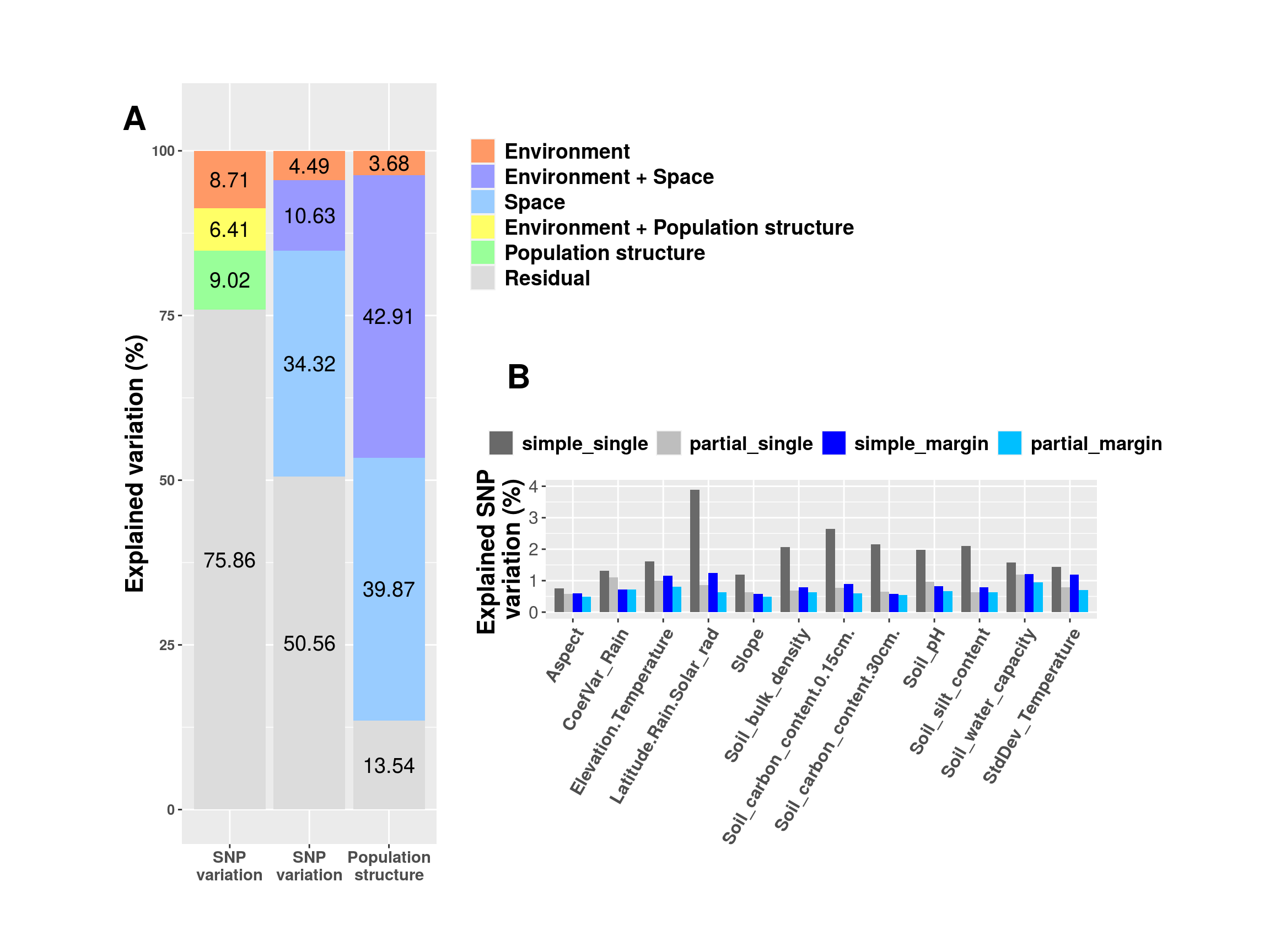
Now, we can look at our results. With the summary table of RDA, we can access the proportion of SNP variation explained by population structure, spatial autocorrelation and environmental variables, respectively. For example, in the summary table of rda.snp.alsQ, we can find that about 15% of variation is explained by the ancestry coefficients (see the column called Proportion).

rda.snp.alsQ

Call: rda(formula = as.matrix(Y) ~ as.matrix(alsQ))

                Inertia Proportion Rank
Total         1.422e+04  1.000e+00     
Constrained   2.194e+03  1.543e-01    3
Unconstrained 1.202e+04  8.457e-01  240
Inertia is variance 
Some constraints were aliased because they were collinear (redundant)

Eigenvalues for constrained axes:
  RDA1   RDA2   RDA3 
1017.5  613.7  562.9 

Eigenvalues for unconstrained axes:
  PC1   PC2   PC3   PC4   PC5   PC6   PC7   PC8 
370.7 309.5 252.5 199.3 195.6 190.6 174.5 169.7 
(Showing 8 of 240 unconstrained eigenvalues)

rda.snp.sp

Call: rda(formula = as.matrix(Y) ~ as.matrix(sel.mem))

                Inertia Proportion Rank
Total         1.422e+04  1.000e+00     
Constrained   6.391e+03  4.495e-01   56
Unconstrained 7.827e+03  5.505e-01  187
Inertia is variance 

Eigenvalues for constrained axes:
 RDA1  RDA2  RDA3  RDA4  RDA5  RDA6  RDA7  RDA8  RDA9 RDA10 RDA11 RDA12 RDA13 
803.8 574.9 484.6 320.6 215.3 182.1 169.3 164.5 156.8 150.7 135.6 128.2 122.2 
RDA14 RDA15 RDA16 RDA17 RDA18 RDA19 RDA20 RDA21 RDA22 RDA23 RDA24 RDA25 RDA26 
116.8 110.6  97.8  95.4  92.7  90.9  89.1  87.3  84.8  81.4  79.4  77.0  76.3 
RDA27 RDA28 RDA29 RDA30 RDA31 RDA32 RDA33 RDA34 RDA35 RDA36 RDA37 RDA38 RDA39 
 73.9  71.4  70.3  69.2  68.1  65.9  63.2  61.1  60.1  58.9  58.5  56.4  55.6 
RDA40 RDA41 RDA42 RDA43 RDA44 RDA45 RDA46 RDA47 RDA48 RDA49 RDA50 RDA51 RDA52 
 54.5  54.1  53.0  52.8  52.0  52.0  50.7  50.4  49.5  49.0  47.7  46.7  46.4 
RDA53 RDA54 RDA55 RDA56 
 44.8  38.0  21.5   7.6 

Eigenvalues for unconstrained axes:
  PC1   PC2   PC3   PC4   PC5   PC6   PC7   PC8 
333.1 222.1 139.5 129.1 117.6 116.0 106.4 104.0 
(Showing 8 of 187 unconstrained eigenvalues)

rda.snp.env

Call: rda(formula = Y ~ Latitude.Rain.Solar_rad + Aspect + Slope +
Elevation.Temperature + Soil_bulk_density + Soil_water_capacity +
Soil_carbon_content.0.15cm. + Soil_carbon_content.30cm. + Soil_pH +
Soil_silt_content + StdDev_Temperature + CoefVar_Rain, data =
predictor)

                Inertia Proportion Rank
Total         1.422e+04  1.000e+00     
Constrained   2.150e+03  1.512e-01   12
Unconstrained 1.207e+04  8.488e-01  231
Inertia is variance 

Eigenvalues for constrained axes:
 RDA1  RDA2  RDA3  RDA4  RDA5  RDA6  RDA7  RDA8  RDA9 RDA10 RDA11 RDA12 
627.7 352.3 254.0 183.9 156.6 113.4  93.5  90.8  76.9  73.6  67.5  59.3 

Eigenvalues for unconstrained axes:
  PC1   PC2   PC3   PC4   PC5   PC6   PC7   PC8 
530.5 466.3 334.8 264.5 237.0 216.1 173.0 160.8 
(Showing 8 of 231 unconstrained eigenvalues)

Three RDA models are significant in the permutation test.

rda.snp.alsQ.anova

Permutation test for rda under reduced model
Permutation: free
Number of permutations: 5000

Model: rda(formula = as.matrix(Y) ~ as.matrix(alsQ))
          Df Variance      F Pr(>F)    
Model      3   2194.1 14.597  2e-04 ***
Residual 240  12024.5                  
---
Signif. codes:  0 '***' 0.001 '**' 0.01 '*' 0.05 '.' 0.1 ' ' 1

rda.snp.sp.anova

Permutation test for rda under reduced model
Permutation: free
Number of permutations: 5000

Model: rda(formula = as.matrix(Y) ~ as.matrix(sel.mem))
          Df Variance      F Pr(>F)    
Model     56   6391.3 2.7267  2e-04 ***
Residual 187   7827.3                  
---
Signif. codes:  0 '***' 0.001 '**' 0.01 '*' 0.05 '.' 0.1 ' ' 1

rda.snp.env.anova

Permutation test for rda under reduced model
Permutation: free
Number of permutations: 5000

Model: rda(formula = Y ~ Latitude.Rain.Solar_rad + Aspect + Slope + Elevation.Temperature + Soil_bulk_density + Soil_water_capacity + Soil_carbon_content.0.15cm. + Soil_carbon_content.30cm. + Soil_pH + Soil_silt_content + StdDev_Temperature + CoefVar_Rain, data = predictor)
          Df Variance      F Pr(>F)    
Model     12   2149.7 3.4288  2e-04 ***
Residual 231  12068.9                  
---
Signif. codes:  0 '***' 0.001 '**' 0.01 '*' 0.05 '.' 0.1 ' ' 1

To calculate adjusted \(R^2\), we can use RsquareAdj function.

RsquareAdj(rda.snp.alsQ)

$r.squared
[1] 0.1543112

$adj.r.squared
[1] 0.1437401

RsquareAdj(rda.snp.sp)

$r.squared
[1] 0.4495023

$adj.r.squared
[1] 0.2846473

RsquareAdj(rda.snp.env)

$r.squared
[1] 0.1511914

$adj.r.squared
[1] 0.1070974

Similarly, we can access the confounded variation by looking at the summary tables. For example, in the summary table of rda.snp.env.sp, we can find that about 45% of variation is explained by MEMs (see the row Conditional) and only 4.5% of variation is exclusively explained by environmental variables.

rda.snp.env.alsQ

Call: rda(formula = Y ~ as.matrix(predictor) +
Condition(as.matrix(alsQ)), scale = F)

                Inertia Proportion Rank
Total         1.422e+04  1.000e+00     
Conditional   2.194e+03  1.543e-01    3
Constrained   1.238e+03  8.710e-02   12
Unconstrained 1.079e+04  7.586e-01  228
Inertia is variance 
Some constraints were aliased because they were collinear (redundant)

Eigenvalues for constrained axes:
  RDA1   RDA2   RDA3   RDA4   RDA5   RDA6   RDA7   RDA8   RDA9  RDA10  RDA11 
204.12 177.36 141.23 119.24 100.27  84.85  82.65  77.01  70.10  66.69  58.73 
 RDA12 
 56.19 

Eigenvalues for unconstrained axes:
   PC1    PC2    PC3    PC4    PC5    PC6    PC7    PC8 
286.55 240.21 225.75 173.28 161.47 157.15 148.16 141.90 
(Showing 8 of 228 unconstrained eigenvalues)

rda.snp.env.sp

Call: rda(formula = as.matrix(Y) ~ as.matrix(predictor) +
Condition(as.matrix(sel.mem)))

                Inertia Proportion Rank
Total         1.422e+04  1.000e+00     
Conditional   6.391e+03  4.495e-01   56
Constrained   6.386e+02  4.491e-02   12
Unconstrained 7.189e+03  5.056e-01  175
Inertia is variance 

Eigenvalues for constrained axes:
  RDA1   RDA2   RDA3   RDA4   RDA5   RDA6   RDA7   RDA8   RDA9  RDA10  RDA11 
135.57  72.64  59.91  50.45  48.26  45.74  41.74  40.52  38.01  36.81  34.58 
 RDA12 
 34.34 

Eigenvalues for unconstrained axes:
   PC1    PC2    PC3    PC4    PC5    PC6    PC7    PC8 
274.41 195.45 135.70 117.92 114.12 104.91 103.22 100.38 
(Showing 8 of 175 unconstrained eigenvalues)

RsquareAdj(rda.snp.env.alsQ)

$r.squared
[1] 0.08709915

$adj.r.squared
[1] 0.04776304

RsquareAdj(rda.snp.env.sp)

$r.squared
[1] 0.04491004

$adj.r.squared
[1] 0.01330805

rda.snp.env.alsQ.anova

Permutation test for rda under reduced model
Permutation: free
Number of permutations: 5000

Model: rda(formula = Y ~ as.matrix(predictor) + Condition(as.matrix(alsQ)), scale = F)
          Df Variance      F Pr(>F)    
Model     12   1238.4 2.1815  2e-04 ***
Residual 228  10786.1                  
---
Signif. codes:  0 '***' 0.001 '**' 0.01 '*' 0.05 '.' 0.1 ' ' 1

rda.snp.env.sp.anova

Permutation test for rda under reduced model
Permutation: free
Number of permutations: 5000

Model: rda(formula = as.matrix(Y) ~ as.matrix(predictor) + Condition(as.matrix(sel.mem)))
          Df Variance      F Pr(>F)    
Model     12    638.6 1.2954  2e-04 ***
Residual 175   7188.8                  
---
Signif. codes:  0 '***' 0.001 '**' 0.01 '*' 0.05 '.' 0.1 ' ' 1

We can further investigate the individual effects and marginal effects of environmental variables.

# make tables summarizing the anova results for all environmental variables (one variable was fitted in an RDA model at a time)
env.names <- names(rda.snp.env.anova.ind)
rda.snp.env.anova.ind <- round(matrix(unlist(lapply(rda.snp.env.anova.ind, function(x){c(x$Df[1], x$Variance[1], x$F[1], x$"Pr(>F)"[1])})), ncol = 4, byrow = T), digits = 4)
rda.snp.env.alsQ.anova.ind <- round(matrix(unlist(lapply(rda.snp.env.alsQ.anova.ind, function(x){c(x$Df[1], x$Variance[1], x$F[1], x$"Pr(>F)"[1])})), ncol = 4, byrow = T), digits = 4)

# name the rows and columns
colnames(rda.snp.env.anova.ind) <- colnames(rda.snp.env.alsQ.anova.ind) <- c("Df", "Variance", "F", "Pr(>F)")
rownames(rda.snp.env.anova.ind) <- rownames(rda.snp.env.alsQ.anova.ind) <- env.names

# individual effects and marginal effects without conditioning on population structure
rda.snp.env.anova.ind

                            Df Variance      F Pr(>F)
Latitude.Rain.Solar_rad      1 553.6372 9.8046  2e-04
Aspect                       1 107.0534 1.8359  2e-04
Slope                        1 170.2299 2.9324  2e-04
Elevation.Temperature        1 229.2979 3.9666  2e-04
Soil_bulk_density            1 293.9198 5.1081  2e-04
Soil_water_capacity          1 225.4961 3.8998  2e-04
Soil_carbon_content.0.15cm.  1 376.0355 6.5739  2e-04
Soil_carbon_content.30cm.    1 306.0195 5.3230  2e-04
Soil_pH                      1 280.3609 4.8677  2e-04
Soil_silt_content            1 298.7987 5.1947  2e-04
StdDev_Temperature           1 204.1527 3.5253  2e-04
CoefVar_Rain                 1 186.4980 3.2164  2e-04

rda.snp.env.anova.bymar

Permutation test for rda under direct model
Marginal effects of terms
Permutation: free
Number of permutations: 5000

Model: rda(formula = Y ~ Latitude.Rain.Solar_rad + Aspect + Slope + Elevation.Temperature + Soil_bulk_density + Soil_water_capacity + Soil_carbon_content.0.15cm. + Soil_carbon_content.30cm. + Soil_pH + Soil_silt_content + StdDev_Temperature + CoefVar_Rain, data = predictor)
                             Df Variance      F    Pr(>F)    
Latitude.Rain.Solar_rad       1    177.1 3.3906 0.0002000 ***
Aspect                        1     85.5 1.6364 0.0017996 ** 
Slope                         1     81.9 1.5674 0.0023995 ** 
Elevation.Temperature         1    164.8 3.1535 0.0002000 ***
Soil_bulk_density             1    112.7 2.1565 0.0002000 ***
Soil_water_capacity           1    171.6 3.2845 0.0002000 ***
Soil_carbon_content.0.15cm.   1    128.0 2.4493 0.0002000 ***
Soil_carbon_content.30cm.     1     81.4 1.5571 0.0053989 ** 
Soil_pH                       1    117.1 2.2410 0.0002000 ***
Soil_silt_content             1    112.0 2.1446 0.0003999 ***
StdDev_Temperature            1    169.4 3.2423 0.0002000 ***
CoefVar_Rain                  1    103.3 1.9776 0.0002000 ***
Residual                    231  12068.9                     
---
Signif. codes:  0 '***' 0.001 '**' 0.01 '*' 0.05 '.' 0.1 ' ' 1

# individual effects and marginal effects controlling the effect of population structure
rda.snp.env.alsQ.anova.ind

                            Df Variance      F Pr(>F)
Latitude.Rain.Solar_rad      1 122.1676 2.4531  2e-04
Aspect                       1  81.2028 1.6250  2e-04
Slope                        1  90.5932 1.8143  2e-04
Elevation.Temperature        1 141.3632 2.8432  2e-04
Soil_bulk_density            1  98.1368 1.9666  2e-04
Soil_water_capacity          1 168.3390 3.3934  2e-04
Soil_carbon_content.0.15cm.  1 110.8457 2.2237  2e-04
Soil_carbon_content.30cm.    1  92.3804 1.8504  2e-04
Soil_pH                      1 136.2396 2.7389  2e-04
Soil_silt_content            1  89.6590 1.7954  2e-04
StdDev_Temperature           1 111.8356 2.2437  2e-04
CoefVar_Rain                 1 156.2026 3.1455  2e-04

rda.snp.env.alsQ.anova.bymar

Permutation test for rda under direct model
Marginal effects of terms
Permutation: free
Number of permutations: 5000

Model: rda(formula = Y ~ Latitude.Rain.Solar_rad + Aspect + Slope + Elevation.Temperature + Soil_bulk_density + Soil_water_capacity + Soil_carbon_content.0.15cm. + Soil_carbon_content.30cm. + Soil_pH + Soil_silt_content + StdDev_Temperature + CoefVar_Rain + Condition(North) + Condition(Coast) + Condition(Eastern_Desert) + Condition(Southern_Desert), data = cbind.data.frame(predictor, alsQ))
                             Df Variance      F    Pr(>F)    
Latitude.Rain.Solar_rad       1     89.2 1.8864 0.0002000 ***
Aspect                        1     69.9 1.4777 0.0089982 ** 
Slope                         1     70.0 1.4805 0.0079984 ** 
Elevation.Temperature         1    114.6 2.4234 0.0002000 ***
Soil_bulk_density             1     89.8 1.8989 0.0005999 ***
Soil_water_capacity           1    134.4 2.8405 0.0002000 ***
Soil_carbon_content.0.15cm.   1     85.1 1.7986 0.0005999 ***
Soil_carbon_content.30cm.     1     77.2 1.6314 0.0033993 ** 
Soil_pH                       1     95.4 2.0162 0.0005999 ***
Soil_silt_content             1     88.7 1.8743 0.0003999 ***
StdDev_Temperature            1    100.3 2.1193 0.0002000 ***
CoefVar_Rain                  1    101.8 2.1510 0.0002000 ***
Residual                    228  10786.1                     
---
Signif. codes:  0 '***' 0.001 '**' 0.01 '*' 0.05 '.' 0.1 ' ' 1

Finally, we visualize the results of variation partitioning.

Version	Author	Date
1202876	Che-Wei Chang	2021-10-22

sessionInfo()

R version 3.6.0 (2019-04-26)
Platform: x86_64-pc-linux-gnu (64-bit)
Running under: Ubuntu 16.04.6 LTS

Matrix products: default
BLAS:   /usr/lib/libblas/libblas.so.3.6.0
LAPACK: /usr/lib/lapack/liblapack.so.3.6.0

locale:
 [1] LC_CTYPE=en_US.UTF-8       LC_NUMERIC=C              
 [3] LC_TIME=en_US.UTF-8        LC_COLLATE=en_US.UTF-8    
 [5] LC_MONETARY=en_US.UTF-8    LC_MESSAGES=en_US.UTF-8   
 [7] LC_PAPER=en_US.UTF-8       LC_NAME=C                 
 [9] LC_ADDRESS=C               LC_TELEPHONE=C            
[11] LC_MEASUREMENT=en_US.UTF-8 LC_IDENTIFICATION=C       

attached base packages:
[1] stats     graphics  grDevices utils     datasets  methods   base     

other attached packages:
[1] ggplot2_3.3.5   vegan_2.5-6     lattice_0.20-38 permute_0.9-5  
[5] vcfR_1.9.0      workflowr_1.6.2

loaded via a namespace (and not attached):
 [1] tidyselect_1.1.1  xfun_0.27         purrr_0.3.4       memuse_4.0-0     
 [5] splines_3.6.0     colorspace_2.0-2  vctrs_0.3.8       generics_0.1.0   
 [9] htmltools_0.5.2   viridisLite_0.4.0 yaml_2.2.1        mgcv_1.8-28      
[13] utf8_1.2.2        rlang_0.4.12      later_1.3.0       pillar_1.6.4     
[17] withr_2.4.2       DBI_1.1.1         glue_1.4.2        lifecycle_1.0.1  
[21] stringr_1.4.0     munsell_0.5.0     gtable_0.3.0      evaluate_0.14    
[25] labeling_0.4.2    knitr_1.36        fastmap_1.1.0     httpuv_1.6.3     
[29] parallel_3.6.0    fansi_0.5.0       highr_0.9         Rcpp_1.0.7       
[33] pinfsc50_1.1.0    promises_1.2.0.1  backports_1.1.5   scales_1.1.1     
[37] farver_2.1.0      fs_1.5.0          digest_0.6.28     stringi_1.7.5    
[41] dplyr_1.0.7       grid_3.6.0        rprojroot_1.3-2   tools_3.6.0      
[45] magrittr_2.0.1    tibble_3.1.5      cluster_2.0.8     crayon_1.4.1     
[49] ape_5.3           whisker_0.4       pkgconfig_2.0.3   ellipsis_0.3.2   
[53] MASS_7.3-51.1     Matrix_1.2-18     assertthat_0.2.1  rmarkdown_2.3    
[57] R6_2.5.1          nlme_3.1-139      git2r_0.26.1      compiler_3.6.0

Partitioning gemomic variation

Che-Wei Chang

2021-10-05

Introduction

Load data

Moran's eigenvector maps (MEMs)

Partitioning SNP variation

Simple RDA

Contribution of population structure

Fit an RDA model

Permutation test

Contribution of spatial autocorrelation

Fit an RDA model

Permutation test

Contribution of all environmental variables

Fit an RDA model

Permutation test

Individual effect of each environmental variable

Marginal effect of each environmental variable

Partial RDA controlling population structure

Total effect of all environmental variables

Fit a partial RDA model

Permutation test

Individual effect of each environmental variable

Marginal effect of each environmental variable

Partial RDA controlling spatial autocorrelation

Total effect of all environmental variables

Fit a partial RDA model

Permutation test

Partitioning population structure

Simple RDA

Contribution of environmental variables

Fit a model

Permutation test

Contribution of spatial autocorrelation

Fit a model

Permutation test

Partial RDA

Contribution of envieonmental variables

Fit a model controlling spatial autocorrelation

Permutation test

Contribution of spatial autocorrelation

Fit a model controlling environmental variables

Permutation test

Results

Partitioning SNP variation