Biogeophysical feedbacks: Daisy World#

Acknowledgements: Code is adapted from a python script by Andrew Bennett

Introduction#

Daisy world is a toy model of the planet designed to show how negative feedbacks with the biosphere can lead to a stable planet temperature over a wide range of solar luminosities. It was introduced by Watson and Lovelock (1983, Tellus B: Chemical and Physical Meteorology 35.4 (1983): 284-289., hereafter WL83) as an example of the Gaia theory, which proposed a solution to the weak young sun paradox. You are also referred to the excellent review paper, Wood et al. (2008), Rev. Geophys.,46, RG1001, doi:10.1029/2006RG000217, referred to W08 hereafter.

In the early stage of the planet, when life had already established, the sun was about 30% weaker than today, and yet mean temperatures must have remained within the rough range of 0-40C which allow life to persist. The Gaia theory proposed a negative, “stabilizing feedback”, whereby the presence of life reduces temperature variability, thus permitted the continued presence of life.

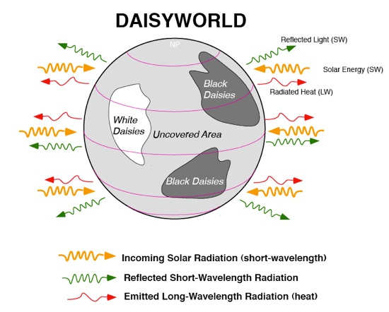
In response to criticism to the theory, WL83 introduced daisy world. Quite simply, a planet is occupied by two species of daisy with different albedos (see figure above), but the same temperature response function where growth is maximized at a certain temperature (22.5C in the paper). Black daisies are warmer than white due to their lower albedo.

The model is simple, consisting of two ODEs that describe the evolution of the black and white daisies as a function of the temperature and three diagnostic equations that describe mean albedo of the planet, the resulting mean temperature assuming energy balance, and the local temperatures of the daisy patches, which are a function of the flower albedo.

Before we start we need to import the modules we will need for the code, numpy and matplotlib for the graphics, and we define a few constants.

Daisy world

Daisyworld image from PSU, David Bice.

The model#

Before we start we need to import the modules we will need for the code, numpy and matplotlib for the graphics, and we define a few constants.

import numpy as np
import matplotlib.pyplot as plt 


keloff=273.15 # to convert between K and deg C 
sigma=5.67e-8 # S-B constant
S0=1000 # solar constant W/m**2
transport=20  # q' in equation 7 of WL83, lineared diffusion heat transport - this relates local albedo perturbations to temperature perturbations
maxloop=100 # number of iterations to allow daisies to equilibrate.
luminosity=np.arange(0.5,1.5,0.01) # range of luminosities ratios over which we will loop, starting from low to high

print (maxloop)

Plant response function#

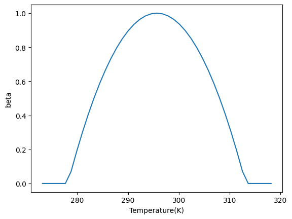
We now define the plant growth temperature response function. This is a quadratic curve that peaks at T=22.5C (you may change this value).

Equation 3 of WL83:

\[ \beta=1-0.003265(22.5-T)^2 \]

The max function ensures positive-definite growth rates, setting the growth rate to zero below about 5C and above 40C. NOTE: Be careful of the units for temperature, which switch between deg C and K in the code and paper.

This plant response function is identical for both kinds of daisies, black and white, thus the difference in growth rates can only be due to their impact on the local temperature due to their albedo.

Let’s code up the temperature response function now, note that we also define the plant death rate, which is introduced in the equations below ($\gamma$):

Td_ideal=22.5+keloff  # peak growth rate for daisies
birth_rate_k=0.003265 #
death_rate=0.3 # fixed death rate gamma in equation 1
def birth_rate(T):
    """function to calculate birth rate"""
    return max(1.0-birth_rate_k*(Td_ideal-T)**2,0.0)

tarr=np.linspace(0,45,41)+keloff
fig,ax=plt.subplots()
br=[birth_rate(t) for t in tarr]
ax.plot(tarr,br)
ax.set_xlabel("Temperature(K)")
ax.set_ylabel("beta")

Text(0, 0.5, 'beta')

The plant function types#

We now introduce some other parameters in the model, the white daisy (dw) and black daisy (db) and bare soil (bs) albedoes:

alb_dw=0.75 # white daisies albedo 
alb_db=0.25 # black daisies
alb_bs=0.5  # bare soil 

We perform the main loop over normalized luminosity values (so L=1 implies present day solar constant), and for each luminosity find the stable solution of daisy area and temperature.

The equations we solve in turn are:

Equation 5 of WL83, this simply states that the mean planetary albedo is an area-weighted average of the daisies and bare soil values.

\[ A_p=A_{dw}\alpha_{dw}+A_{db}\alpha_{db}+A_{bs}\alpha_{bs} \]

where $\alpha$ is the fractional coverage of the white daisies (dw), black daises (db) or bare soil (bs) and $A$ is the respective albedo of each land cover type. (NOTE: We use this notation to follow WL83 and W08, but do not get confused as we usually use $\alpha$ for albedo in the course).

We then calculate the planet mean temperature, which is a simple energy balance equation between incoming solar and emitted infrared radiation (Equation 4 of WL83) (note they are ignoring the emissivity of the grey atmosphere for simplicity, here the atmosphere is transparent to SW and IR radn, it doesn’t really change anything in the behaviour of the model).

\[ T_e=\sqrt[4]{\frac{LS_0(1-A_p)}{\sigma}} \]

The next step is to calculate the local temperature resulting from the presence of the daisies. In WL83 this is not explained in much detail, and we thus refer to the excellent description of W08: The local temperatures $T_{dw}$ and $T_{db}$ and the bare soil temperature $T_{bs}$ are defined by making a simplifying assumption about the heat transfer, essentially a linearization of adiffusion term (refer to the 1D zonal model for ice albedo feedback). This gives a degree of connectedness to the daisy patches without introducing space explicitly. A parameter $q$ is defined as the heat transfer coefficient in WL83, thereby defining the local temperatures as (equation 7 of WL83 or 5-7 in W08):

\[ T_{dw}=q(A_p-A_{dw})+T_e \]

and similarly for the black daisies.

Now we only have to define the two key equations, which describe the birthrate of each daisy type which is a function of their optimum temperatures, using the birthrate function defined above. Each daisies has a constant death rate $\gamma$, converting daisy coverage back to bare soil. These equations are standard for population dynamics, disease models etc. These are eqn. 1 in WL83 or eqn 2 in W08:

\[ \frac {\partial \alpha_{dw}}{\partial t}=\alpha_{dw}(\alpha_{bs}\beta(T_{dw})-\gamma) \]

\[ \frac {\partial \alpha_{db}}{\partial t}=\alpha_{db}(\alpha_{bs}\beta(T_{db})-\gamma) \]

In the code below we note the solver is not accurate, as the system is coupled and the integration method is explicit, but it simple to understand and will do for present purposes. If you have finished the ICTP diploma course in numerical methods I/II you may like to replace this, implementing a Runge-Kutta 4th order solver for example.

# store arrays 
area_dw_v=[]
area_db_v=[]
area_bs_v=[]
T_p_v=[]
T_ref=[]

area_dw=area_db=0.01 # initial conditions

#luminosity=[1]

# loop over luminosity...
for iflux,flux in enumerate(luminosity):
    # initial conditions are taken from a previous run, subject to 
    # a minimum of 1% in case the species had died out 
    area_dw=max(area_dw,0.01)   # white daisies can't die out
    area_db=max(area_db,0.01)   # black daises neither  
    area_bs=1.0-area_dw-area_db # bare soil fraction
    delta_db=delta_dw=1
    
    iloop=0 
    
    while (abs(delta_db)+abs(delta_dw))>1.e-8:
        iloop+=1
        
        # EQN 5: calculate weighted average albedo
        alb_p=area_dw*alb_dw+area_db*alb_db+area_bs*alb_bs
        
        # EQN 4: calculate planet mean temperature
        T_p=np.power(flux*S0*(1-alb_p)/sigma,0.25)
         
        # EQN 7: calculate local temperatures
        T_db=transport*(alb_p-alb_db)+T_p
        T_dw=transport*(alb_p-alb_dw)+T_p
        
        # EQN 3: calculate birth rate beta
        birth_rate_db=birth_rate(T_db)
        birth_rate_dw=birth_rate(T_dw)
           
        # EQN 1: change in daisy area
        delta_db=area_db*(birth_rate_db*area_bs-death_rate)
        delta_dw=area_dw*(birth_rate_dw*area_bs-death_rate)
        area_db+=delta_db
        area_dw+=delta_dw
        
        # update areas
        area_bs=1.0-area_db-area_dw

        #print (area_db,area_dw,area_bs)
     
    print (flux," converged after iteration ",iloop)
    # store the value...
    area_db_v.append(area_db)
    area_dw_v.append(area_dw)
    area_bs_v.append(area_bs)
    T_p_v.append(T_p)
    T_ref.append(np.power(flux*S0*(1-alb_bs)/sigma,0.25))

5  converged after iteration  39
51  converged after iteration  39
52  converged after iteration  39
53  converged after iteration  39
54  converged after iteration  39
55  converged after iteration  39
56  converged after iteration  39
5700000000000001  converged after iteration  39
5800000000000001  converged after iteration  39
5900000000000001  converged after iteration  39
6000000000000001  converged after iteration  39
6100000000000001  converged after iteration  39
6200000000000001  converged after iteration  39
6300000000000001  converged after iteration  39
6400000000000001  converged after iteration  58
6500000000000001  converged after iteration  134
6600000000000001  converged after iteration  52
6700000000000002  converged after iteration  633
6800000000000002  converged after iteration  2165
6900000000000002  converged after iteration  556
7000000000000002  converged after iteration  314
7100000000000002  converged after iteration  218
7200000000000002  converged after iteration  169
7300000000000002  converged after iteration  139
7400000000000002  converged after iteration  119
7500000000000002  converged after iteration  104
7600000000000002  converged after iteration  93
7700000000000002  converged after iteration  84
7800000000000002  converged after iteration  78
7900000000000003  converged after iteration  72
8000000000000003  converged after iteration  68
8100000000000003  converged after iteration  64
8200000000000003  converged after iteration  61
8300000000000003  converged after iteration  58
8400000000000003  converged after iteration  56
8500000000000003  converged after iteration  55
8600000000000003  converged after iteration  53
8700000000000003  converged after iteration  52
8800000000000003  converged after iteration  52
8900000000000003  converged after iteration  51
9000000000000004  converged after iteration  51
9100000000000004  converged after iteration  51
9200000000000004  converged after iteration  51
9300000000000004  converged after iteration  52
9400000000000004  converged after iteration  52
9500000000000004  converged after iteration  53
9600000000000004  converged after iteration  54
9700000000000004  converged after iteration  55
9800000000000004  converged after iteration  57
9900000000000004  converged after iteration  58
0000000000000004  converged after iteration  60
0100000000000005  converged after iteration  62
0200000000000005  converged after iteration  64
0300000000000005  converged after iteration  66
0400000000000005  converged after iteration  69
0500000000000005  converged after iteration  72
0600000000000005  converged after iteration  76
0700000000000005  converged after iteration  79
0800000000000005  converged after iteration  84
0900000000000005  converged after iteration  89
1000000000000005  converged after iteration  94
1100000000000005  converged after iteration  100
1200000000000006  converged after iteration  108
1300000000000006  converged after iteration  116
1400000000000006  converged after iteration  126
1500000000000006  converged after iteration  138
1600000000000006  converged after iteration  152
1700000000000006  converged after iteration  170
1800000000000006  converged after iteration  192
1900000000000006  converged after iteration  222
2000000000000006  converged after iteration  264
2100000000000006  converged after iteration  325
2200000000000006  converged after iteration  426
2300000000000006  converged after iteration  628
2400000000000007  converged after iteration  1248
2500000000000007  converged after iteration  3058
2600000000000007  converged after iteration  876
2700000000000007  converged after iteration  533
2800000000000007  converged after iteration  387
2900000000000007  converged after iteration  305
3000000000000007  converged after iteration  251
3100000000000007  converged after iteration  214
3200000000000007  converged after iteration  186
3300000000000007  converged after iteration  164
3400000000000007  converged after iteration  146
3500000000000008  converged after iteration  131
3600000000000008  converged after iteration  119
3700000000000008  converged after iteration  108
3800000000000008  converged after iteration  98
3900000000000008  converged after iteration  89
4000000000000008  converged after iteration  81
4100000000000008  converged after iteration  74
4200000000000008  converged after iteration  67
4300000000000008  converged after iteration  71
4400000000000008  converged after iteration  61
4500000000000008  converged after iteration  39
4600000000000009  converged after iteration  39
4700000000000009  converged after iteration  39
4800000000000009  converged after iteration  39
4900000000000009  converged after iteration  39

Results#

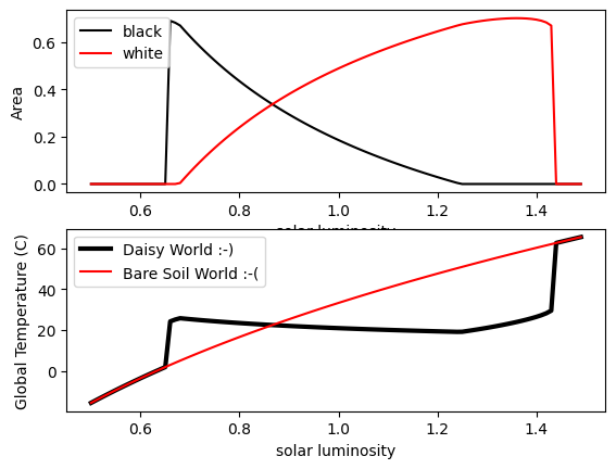
Now we just need to plot the results:

fig,ax=plt.subplots(2,1)
ax[0].plot(luminosity,area_db_v,color='black',label='black')
ax[0].plot(luminosity,area_dw_v,color='red',label='white')
ax[0].set_xlabel('solar luminosity')
ax[0].set_ylabel('Area')
ax[0].legend(loc="best")

ax[1].plot(luminosity,np.array(T_p_v)-keloff,color="black",label="Daisy World :-)",linewidth=3)
ax[1].plot(luminosity,np.array(T_ref)-keloff,color="red",label="Bare Soil World :-(")
ax[1].set_xlabel('solar luminosity')
ax[1].set_ylabel('Global Temperature (C)')
ax[1].legend()

<matplotlib.legend.Legend at 0x1140e1a50>

We see the very interesting behaviour of daisy world. Once the black daisies are established, they locally increase the temperature, and as the luminosity increases in also allows white daisies to be established. Increases in luminosity in turn increase the proportion of white daisies, which reduce the local temperature due to the higher albedo (note, higher than bare soil). The key take home of WL83 was that, relative to bare soil world (red line) the temperature is very stable. In fact you will see when you carry out some of the exercises below that the two daisies type are actually mutually beneficial in the standard set up of these model, that is “cooperative”, and can coexist across a far wider range of luminosity than is the case when a single species exists. This perhaps has important implications for the importance of biodiversity on our planet!

Questions to investigate#

What happens if you change the albedo values of the black and/or white daisies? Try altering the albedos but keeping $A_{db} < A_{bs} < A_{dw}$. But then also try $A_{db} < A_{dw} < A_{bs}$ or $A_{bs} < A_{db} < A_{dw}$.
Tinker with the daisy-dependent death rates and see what happens
What happens if, after arriving at a luminosity $L$ of 1.6 you turn the sun back down again? (i.e. reverse the luminosity loop). Do the solution branches follow each other exactly, or is there a hysteresis? Why?
What happens if for each value of luminosity you start from a near bare earth? (1% coverage for each daisy type) At which values of luminosity does the population crash occur?
What happens if you only allow one daisy type?
What happens if you introduce 3 (or more) daisy types?
Watson and Lovelock introduce another experiment in which black daisies are warmer, but they cool the planet by introducing clouds. This experiment can be conducted by assuming that the TOA albedo for black daisy areas is 0.8, the daises are still warmer than white daisies due to their lower albedo (not very physical!) - See if you can reproduce fig 2 of Watson and Lovelock with this experiment. What happens to the white daisies?
Can you introduce adaptation? You could apply random mutations to the constants in the $\beta$ plant growth function over time, perhaps introduces to a third type with a seed fraction at a particular time.

Have fun and above all, never stop asking yourself “what if?”

Earth System Modelling

Biogeophysical feedbacks: Daisy World

Contents