Last updated: 2021-10-22

Checks: 5 2

Knit directory: Barley1kGBS_Proj/

This reproducible R Markdown analysis was created with workflowr (version 1.6.2). The Checks tab describes the reproducibility checks that were applied when the results were created. The Past versions tab lists the development history.

R Markdown file: uncommitted changes

The R Markdown file has unstaged changes. To know which version of the R Markdown file created these results, you'll want to first commit it to the Git repo. If you're still working on the analysis, you can ignore this warning. When you're finished, you can run wflow_publish to commit the R Markdown file and build the HTML.

Environment: empty

Great job! The global environment was empty. Objects defined in the global environment can affect the analysis in your R Markdown file in unknown ways. For reproduciblity it's best to always run the code in an empty environment.

Seed: set.seed(20210831)

The command set.seed(20210831) was run prior to running the code in the R Markdown file. Setting a seed ensures that any results that rely on randomness, e.g. subsampling or permutations, are reproducible.

Session information: recorded

Great job! Recording the operating system, R version, and package versions is critical for reproducibility.

Cache: detected

The following chunks had caches available:

unnamed-chunk-10
unnamed-chunk-11
unnamed-chunk-12
unnamed-chunk-14
unnamed-chunk-15
unnamed-chunk-16
unnamed-chunk-4
unnamed-chunk-5
unnamed-chunk-6
unnamed-chunk-7
unnamed-chunk-8
unnamed-chunk-9

To ensure reproducibility of the results, delete the cache directory GenomeEnvAssociation_cache and re-run the analysis. To have workflowr automatically delete the cache directory prior to building the file, set delete_cache = TRUE when running wflow_build() or wflow_publish().

File paths: relative

Great job! Using relative paths to the files within your workflowr project makes it easier to run your code on other machines.

Repository version: 43eb596

Great! You are using Git for version control. Tracking code development and connecting the code version to the results is critical for reproducibility.

The results in this page were generated with repository version 43eb596. See the Past versions tab to see a history of the changes made to the R Markdown and HTML files.

Note that you need to be careful to ensure that all relevant files for the analysis have been committed to Git prior to generating the results (you can use wflow_publish or wflow_git_commit). workflowr only checks the R Markdown file, but you know if there are other scripts or data files that it depends on. Below is the status of the Git repository when the results were generated:


Ignored files:
    Ignored:    .Rhistory
    Ignored:    .Rproj.user/
    Ignored:    analysis/GenomeEnvAssociation_cache/
    Ignored:    analysis/GenomicVarPartitioning_cache/
    Ignored:    analysis/PreprocessEnvData_cache/

Untracked files:
    Untracked:  analysis/not_show/
    Untracked:  code/Rfunctions.R
    Untracked:  code/rename_IDs_and_env.R
    Untracked:  data/2020-04-09-simple_rda_single_env_anova_5000perm.RDS
    Untracked:  data/2020-04-10-partial_rda_ALStructure_K4_ancestry_coeff_anova_5000perm_191B1K+53KS_12envs_27147SNPs_maf0.05.RDS
    Untracked:  data/2020-04-10-partial_rda_conditioning_ancestry_coeff_191B1K+53KS_single_env_anova_5000perm.RDS
    Untracked:  data/2020-04-10-simple_rda_anova_5000perm_191B1K+53KS_12envs_27147SNPs_maf0.05.RDS
    Untracked:  data/2020-04-10-simple_rda_anova_5000perm_bymargin_191B1K+53KS_12envs_27147SNPs_maf0.05.RDS
    Untracked:  data/2020-04-11-partial_rda_ALStructure_K4_ancestry_coeff_anova_5000perm_bymargin_191B1K+53KS_12envs_27147SNPs_maf0.05.RDS
    Untracked:  data/2020-04-12-simple_rda_ancescoeff_anova_5000perm_191B1K+53KS_271472SNPs_maf0.05.RDS
    Untracked:  data/2020-04-13-simple_rda_ancescoeff_vs_env_anova_5000perm_191B1K+53KS.RDS
    Untracked:  data/2021-05-30-partial_rda_ancescoeff_vs_env_conditioning_fwselMEM_anova_5000perm_191B1K+53KS.RDS
    Untracked:  data/2021-05-30-partial_rda_fwselMEM_anova_5000perm_191B1K+53KS_12envs_27147SNPs_maf0.05.RDS
    Untracked:  data/2021-05-30-simple_rda_ancescoeff_vs_fwselMEM_anova_5000perm_191B1K+53KS.RDS
    Untracked:  data/2021-05-30-simple_rda_fwselMEM_anova_5000perm_191B1K+53KS_no_envs_27147SNPs_maf0.05.RDS
    Untracked:  data/Ancestry_coeff_244accessions_ALStructure_K4.RDS
    Untracked:  data/Env_data_244accessions_12Env_variables.tsv
    Untracked:  data/Full_MEM_191B1K+53KS.tsv
    Untracked:  data/GBS_244accessions_27147SNP_Beagle5Imp.vcf.gz
    Untracked:  data/GBS_244accessions_LDpruned_19601SNP.vcf.gz
    Untracked:  data/ISR_SRTM_GeoElevation.tif
    Untracked:  data/RawEnv_244accessions.tsv
    Untracked:  data/dbMEM_forward_selection_SNPvsFullMEM.RDS
    Untracked:  data/geo_coordinates_244accessions.tsv

Unstaged changes:
    Modified:   .Rprofile
    Modified:   .gitattributes
    Modified:   .gitignore
    Modified:   Barley1kGBS_Proj.Rproj
    Modified:   README.md
    Modified:   _workflowr.yml
    Modified:   analysis/GenomeEnvAssociation.Rmd
    Modified:   analysis/_site.yml
    Modified:   analysis/about.Rmd
    Modified:   code/README.md
    Modified:   data/README.md
    Modified:   output/README.md

Note that any generated files, e.g. HTML, png, CSS, etc., are not included in this status report because it is ok for generated content to have uncommitted changes.

These are the previous versions of the repository in which changes were made to the R Markdown (analysis/GenomeEnvAssociation.Rmd) and HTML (docs/GenomeEnvAssociation.html) files. If you've configured a remote Git repository (see ?wflow_git_remote), click on the hyperlinks in the table below to view the files as they were in that past version.

File	Version	Author	Date	Message
html	43eb596	Che-Wei Chang	2021-10-22	Build site.
Rmd	7c6b41a	Che-Wei Chang	2021-10-22	wflow_publish(list.files("./analysis", pattern = "*.Rmd", full.names = T))

Introduction

To identify genomic regions that potentially under environmental selection, we perform genome scan with genome-environment association (GEA) approaches.

Here, we use three approaches, including (1) simple RDA (2) partial RDA controlling population structure, and (3) LFMM (Caye et al. 2019). Two RDA approaches assumes that environmental selection gradients do not result from single environmental variables but a combination of environmental variables. In contrast, LFMM is a single-variate approach that consider one environmental variable at a time.

Genomic scan with RDA

To know more details of RDA approach, please check Lasky et al. (2012) and Forester et al. (2018). We use the statistical framework proposed by Capblancq et al. (2018) to carry out statistical tests for RDA.

Briefly, in the framework of Capblancq et al. (2018), we first select the most informative K axes of the RDA according to the plot of the explained variation with the "elbow" method. Subsequently, Mahalanobis distance is calculated for each SNP locus (adaptive SNPs are expected to diverge from the majority of SNPs, so they should have large Mahalanobis distances). To obtain p-values, Mahalanobis distances are divided by the genomic inflation factor to approximate a chi-squared distribution with K degree of freedom (see Luu et al. 2017). The genomic inflation factor is a constant defined as he median of the Mahalanobis distances divided by the median of the chi-square distribution with K degrees of freedom (Luu et al. 2017). Finally, statistical tests can be carried out based on the chi-squared distribution with K degree of freedom.

Load data

rm(list = ls())
source("./code/Rfunctions.R")

library(vcfR)
library(vegan)
 
# load genotypic data (244 accessions with 27,147 SNPs imputed by Beagle 5 with defaults)
geno <- read.vcfR("./data/GBS_244accessions_27147SNP_Beagle5Imp.vcf.gz", verbose = F)
Y <- t(vcf_to_nummatrix(geno))
colnames(Y) <- geno@fix[,"ID"]


CHR <- as.numeric(geno@fix[,"CHROM"])
POS <- as.numeric(geno@fix[,"POS"])

# load environmental data (244 accessions with 12 environmental variables)
env <- read.delim("./data/Env_data_244accessions_12Env_variables.tsv", header = T)
predictor <- as.data.frame(scale(env)) # standardize data

# load ancestry coefficients (K=4) estimated with ALStructure (https://doi.org/10.1534/genetics.119.302159)
alsQ <- t(readRDS("./data/Ancestry_coeff_244accessions_ALStructure_K4.RDS")$Q_hat)


# perform PCA
vcf <- read.vcfR("./data/GBS_244accessions_LDpruned_19601SNP.vcf.gz", verbose = F) # this vcf is LD prunned and unimputed, which is for population structure analysis.
Xmat <- vcf_to_nummatrix(vcf = vcf)
impX <- t(apply(Xmat,1,function(x){
  x[is.na(x)] <- mean(x, na.rm = T) 
  return(x)
}))

barley.pc <- prcomp(t(impX))

RDA approaches

Simple RDA

rda.snp.env <- rda(as.formula(paste("Y ~ ",paste(colnames(predictor), collapse = " + "), sep = "")), data = predictor)

Partial RDA controlling population structure

rda.snp.env.alsQ <- rda(Y ~ as.matrix(predictor) + Condition(as.matrix(alsQ)), scale = F)

PCs <- barley.pc$x[,1:3] # choose the first three PC axes to represent population structure
rda.snp.env.pc <- rda(Y ~ as.matrix(predictor) + Condition(as.matrix(PCs)), scale = F)

Selection of K

To determine the number of RDA axes for calculating Mahalanobis distance, we make a plot showing the proportion of explained variation of each axis. As there is no very conspicuous "elbow" in the plot, I choose K=4, which is the least K in the interval where "elbow" appears in the curve of the simple RDA.

library(ggplot2)
dat <- data.frame("K"=as.factor(rep(1:12, times = 3)),"Exp_prop" = c(summary(rda.snp.env)$concont[[1]][2,], summary(rda.snp.env.alsQ)$concont[[1]][2,], summary(rda.snp.env.pc)$concont[[1]][2,]
                                                                     ), "model" = rep(c("Simple_RDA", "RDA_Als", "RDA_PC"), each = 12))

ggplot(dat, aes(x=K, y=Exp_prop, group=model)) +
  geom_line(aes(linetype=model)) + 
  geom_point() +
  ylab("Explained proportion")

Statistical test

To conduct statistical tests, we use the R function rdadapt (see github.com/Capblancq/RDA-genome-scan). This function returns both p-values and q-values.

# load libraries required for rdadapt
library(robust)
library(qvalue)

k = 4 # number of RDA axes to retain
rda.simple.pq <- rdadapt(rda.snp.env, K = k)
rda.partial.alsQ.pq <- rdadapt(rda.snp.env.alsQ, K = k)
rda.partial.pc.pq <- rdadapt(rda.snp.env.pc, K = k)

Differences between using ancestry coefficients and PCs

As we use two approaches to condition an RDA model on population structure (ancestry coefficients and PC scores), it is interesting to look at how different between the results of them.

We further zoom-in to those SNPs with q-values < 0.05.

Here we check how many SNPs are significant in a partial RDA model but not significant in another.

# the number of SNPs significant in the RDA conditioned on ancestry coefficients but not on PCs
sum(rda.partial.alsQ.pq$q.values <= 0.05 & rda.partial.pc.pq$q.values > 0.05)

[1] 7

# the number of SNPs significant in the RDA conditioned on PCs but not on ancestry coefficients
sum(rda.partial.alsQ.pq$q.values > 0.05 & rda.partial.pc.pq$q.values <= 0.05)

[1] 19

By comparing the results of two approaches, we confirmed there is only very little difference between conditioned on ancestry coefficients and PC scores. A possible explanation for this is that ALStructure is a method bridging PCA with the model-based population structure analysis (like STRUCTURE and ADMIXTURE). For the downstream analysis, we would only show the results of RDA conditioned on ancestry coefficients.

We take FDR = 0.05 as a significance level for statistical tests.

Simple RDA

Partial RDA controlling population structure

LFMM

library(lfmm)
fit.lfmm <- lfmm_ridge(Y = Y, X = predictor, K = 4)

pv <- lfmm_test(Y = Y, X = predictor, lfmm = fit.lfmm, 
                calibrate = "gif")

pvalues <- pv$calibrated.pvalue 

# check if the distribution of p-value agree with the FDR assumption
hist(as.vector(pvalues), xlab = "Adjusted P-values", main = "Distribution of Adjusted P-values of LFMM (K = 4)")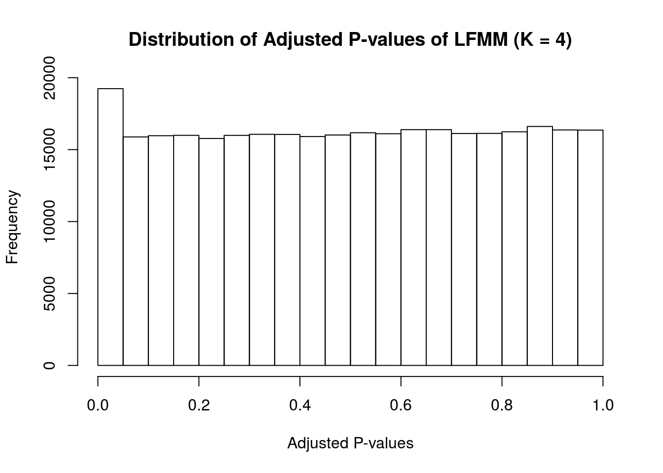

Version	Author	Date
43eb596	Che-Wei Chang	2021-10-22

# calculate q-value for each GEA test respectively
qvalues <- 
  apply(pvalues,2, function(x){
    qvalue(x)$qvalues
  })

rownames(qvalues) <- rownames(pvalues)
colnames(qvalues) <- colnames(pvalues)

Number of significant SNPs

For all environmental variables

There are 307 significant SNPs in total for all environmental variables.

sum(apply(qvalues, 1, function(x){any(x < 0.05)}))

[1] 307

For each environmental variable

We further look at the number of significant SNPs for each environmental variable.

Env	Number_of_SNPs
Latitude.Rain.Solar_rad	4
Aspect	0
Slope	0
Elevation.Temperature	108
Soil_bulk_density	0
Soil_water_capacity	1
Soil_carbon_content.0.15cm.	11
Soil_carbon_content.30cm.	0
Soil_pH	2
Soil_silt_content	0
StdDev_Temperature	179
CoefVar_Rain	12

Manhattan plots of LFMM

sessionInfo()

R version 3.6.0 (2019-04-26)
Platform: x86_64-pc-linux-gnu (64-bit)
Running under: Ubuntu 16.04.6 LTS

Matrix products: default
BLAS:   /usr/lib/libblas/libblas.so.3.6.0
LAPACK: /usr/lib/lapack/liblapack.so.3.6.0

locale:
 [1] LC_CTYPE=en_US.UTF-8       LC_NUMERIC=C              
 [3] LC_TIME=en_US.UTF-8        LC_COLLATE=en_US.UTF-8    
 [5] LC_MONETARY=en_US.UTF-8    LC_MESSAGES=en_US.UTF-8   
 [7] LC_PAPER=en_US.UTF-8       LC_NAME=C                 
 [9] LC_ADDRESS=C               LC_TELEPHONE=C            
[11] LC_MEASUREMENT=en_US.UTF-8 LC_IDENTIFICATION=C       

attached base packages:
[1] stats     graphics  grDevices utils     datasets  methods   base     

other attached packages:
[1] lfmm_0.0          qvalue_2.16.0     robust_0.4-18.2   fit.models_0.5-14
[5] vegan_2.5-6       lattice_0.20-38   permute_0.9-5     vcfR_1.9.0       

loaded via a namespace (and not attached):
 [1] viridisLite_0.3.0   splines_3.6.0       foreach_1.4.7      
 [4] memuse_4.0-0        stats4_3.6.0        yaml_2.2.1         
 [7] robustbase_0.93-5   pillar_1.6.1        backports_1.1.5    
[10] glue_1.4.2          RcppEigen_0.3.3.7.0 digest_0.6.25      
[13] promises_1.1.1      colorspace_1.4-1    htmltools_0.5.1.1  
[16] httpuv_1.5.4        Matrix_1.2-18       plyr_1.8.5         
[19] pcaPP_1.9-73        pkgconfig_2.0.3     purrr_0.3.3        
[22] mvtnorm_1.0-12      scales_1.1.0        whisker_0.4        
[25] RSpectra_0.16-0     later_1.1.0.1       git2r_0.26.1       
[28] tibble_2.1.3        mgcv_1.8-28         generics_0.0.2     
[31] ggplot2_3.3.2       ellipsis_0.3.2      magrittr_1.5       
[34] crayon_1.3.4        evaluate_0.14       fs_1.5.0           
[37] fansi_0.4.1         nlme_3.1-139        MASS_7.3-51.1      
[40] tools_3.6.0         lifecycle_1.0.0     stringr_1.4.0      
[43] munsell_0.5.0       cluster_2.0.8       compiler_3.6.0     
[46] rlang_0.4.11        grid_3.6.0          iterators_1.0.12   
[49] rstudioapi_0.13     rmarkdown_2.3       gtable_0.3.0       
[52] codetools_0.2-16    DBI_1.1.0           reshape2_1.4.3     
[55] rrcov_1.5-2         R6_2.4.1            knitr_1.29         
[58] dplyr_1.0.6         pinfsc50_1.1.0      utf8_1.1.4         
[61] workflowr_1.6.2     rprojroot_1.3-2     ape_5.3            
[64] stringi_1.5.3       parallel_3.6.0      Rcpp_1.0.5         
[67] vctrs_0.3.8         DEoptimR_1.0-8      tidyselect_1.1.1   
[70] xfun_0.17

Genome-Environment Association

Che-Wei Chang

2021-10-05

Introduction

Genomic scan with RDA

Load data

RDA approaches

Simple RDA

Partial RDA controlling population structure

Selection of K

Statistical test

Differences between using ancestry coefficients and PCs

Simple RDA

Partial RDA controlling population structure

LFMM

Number of significant SNPs

For all environmental variables

For each environmental variable

Manhattan plots of LFMM